

Memory Management#
Gary L. Pavlis and Ian (Yinzhi) Wang
Overview#
Dask and Spark, which are used in MsPASS to exploit parallel processing, are generic packages to implement the map-reduce paradigm of parallel processing. As generic frameworks Dask and Spark are flexible but not as efficient and bombproof as a typical seismic reflection processing package. One of the biggest weaknesses we have found with these packages is default memory management can lead to poor performance or, in the worst case, memory faults. The biggest problem seems to be when the size of the data objects considered atomic (Components of the generalized list called an RDD by Spark and a bag by Dask) are a significant fraction of any nodes memory.
In this document we discuss pitfalls we are aware of in memory management with MsPASS. This document is focused mainly on dask because we have more experience using it. The main dask document on dask memory management is found here. The comparable page for spark is here. As for most heavily used packages like this there are also numerous pages on the topic that will quickly bury you with a web search. We produced this document to help you wade through the confusion by focusing on the practical experience with MsPASS. When we are talking specifically about dask or spark we will say so. We will use the term scheduler to refer to generic concepts common to both.
WARNING: This is an evolving topic the authors of MsPASS are continuing to evaluate. Treat any conclusions in this document with skepticism.
DAGs, tasks, and the map-reduce model of processing#
To understand the challenge a scheduler faces in processing a workflow, and memory management we need to digress a bit and review the way a scheduler operates. Dask and spark both abstract processing as a sequence of “tasks”. A “task” in this context is more-or-less the operation defined in a particular call to a “map” or “reduce” operator. (If you are unfamiliar with this concept see section Parallel Processing and/or a web search for a tutorial on the topic.) Each “task” can be visualized as a black box that takes one or more inputs and emits an output. Since in a programming language that is the same thing conceptually as a “function call” map and reduce operators always have a function object as one of the arguments. A “map” operator has one main input (arguments to the function are auxiliary data) and a single output (the function return). Reduce operators have many inputs of a common data type and one output. Note, however, the restriction that they are always considered two at a time. For most MsPASS operators the inputs and outputs are seismic data objects. The only common exception is constructs used to provide inputs to readers such as when read_distributed_data is used to load ensembles.
Dask and spark both abstract the job they are asked to handle as a tree structure called a “Directed Acyclic Graph” (DAG). The nodes of the tree are individual “tasks”. It has been our experience that most workflows end up being only a sequence of map operators. In that case, the DAG reduces to a forest of saplings (sticks with no branches) with the first task being a read operation and the last being a write (save) operation.
To clarify that abstract idea consider a concrete example. The code box below is a dask implementation of a simple job with 7 steps: query database to define the dataset, read data, detrend, bandpass filter, window around P arrival time, compute signa-to-noise estimates, and save result. Here is a sketch of the workflow omitting complexities of imports and initializations:
# assume database handle, db, and query are defined earlier
cursor = db.wf_miniseed.find(query)
# Npartitions assumed defined in initializations - see text below for
# what this defines and why it is important for memory management
mybag = read_distributed_data(db,cursor,npartitions=Npartitions)
mybag = mybag.map(detrend)
mybag = mybag.map(filter,type="bandpass",freqmin=0.01,freqmax=1.5)
mybag = mybag.map(WindowData,-200.0,200.0)
# assume nwin and swin defined initialization
mybag = mybag.map(arrival_snr,noise_window=nwin,signal_window=swin)
mybag = mybag.map(db.save_data,data_tag="step1",return_data=False)
mybag.compute()
This simple workflow consists only of map operators and is terminated by a save followed by a compute to initiate the (lazy) computation of the bag. The DAG for this workflow is illustrated below
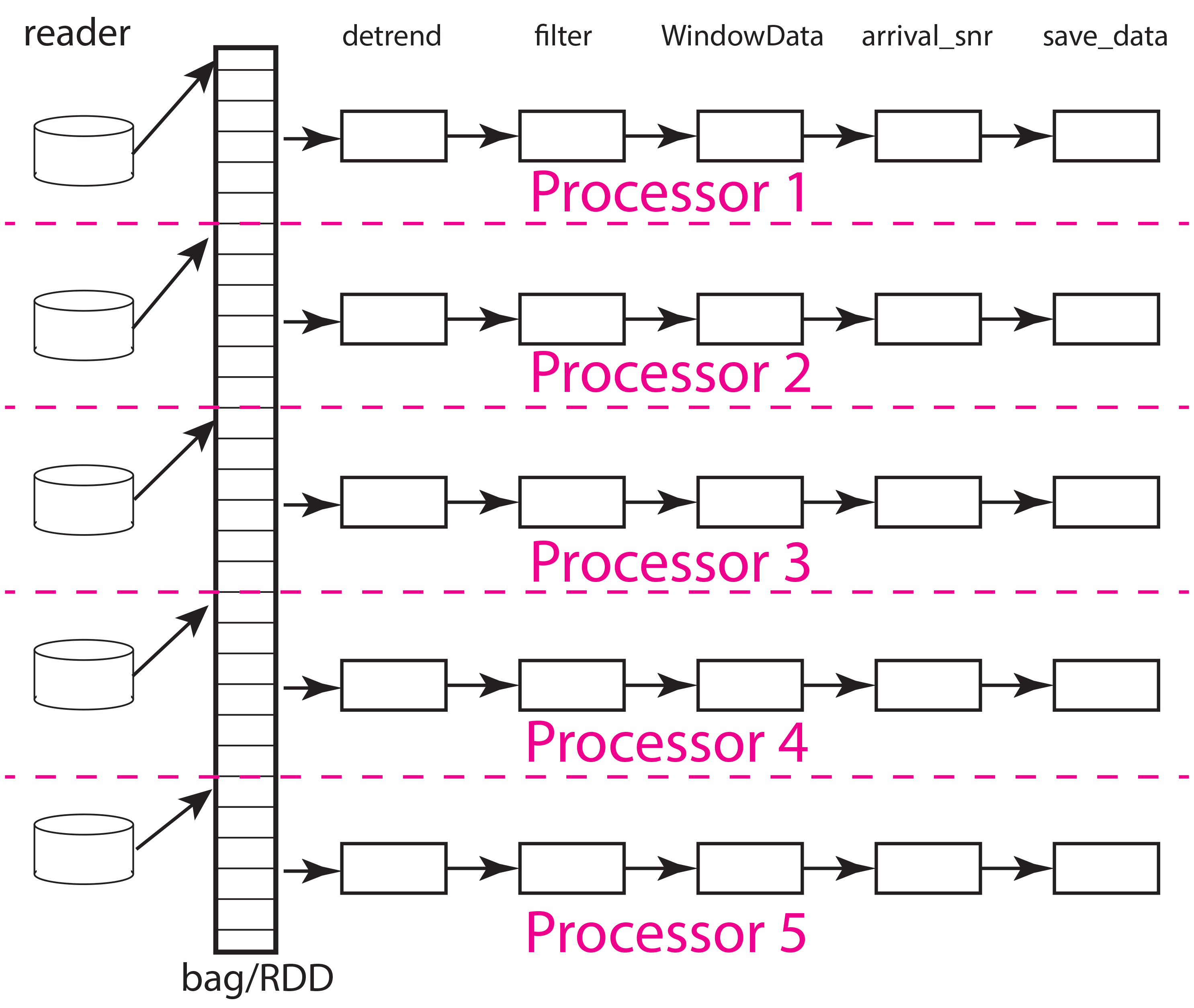
Fig. 18 Block diagram illustration of DAG defined by example workflow. The example shows how work would be partitions with five processors and five partitions. The labels at the top are function names matching those used in the python code above. Each box denotes an instance of that function run on one processor (worker). Data flow is from left to right. Data enter each pipeline from a reader on the left hand side (read_distributed_data but here given the simpler name “reader”) and exit in the save operation. For this simple case where the number of processors match the number of partitions each processor would be assigned 1/5th of the data. Termination of the workflow with a database save (save_data) makes each pipeline largely independent of the others and can improve performance as not processor has to wait for another except in competition for attention from the database server.#
Now remember that a bag (RDD in spark) can be conceptualized as a container that is a list of data objects that doesn’t necessarily fit into cluster memory, let alone a single node. Both dask and spark divide the container into partitions illustrated in the figure above. The partition size can be as small as one data object or some larger integer less than or equal to the number of data components. Think of a partition as the size of a bite the system uses to eat the elephant (the whole data set). That basic understanding should help you immediately realize that the partition size relative to system memory is a critical tuning component to optimize performance and make a workflow feasible. Setting the number of partitions too large can overwhelm the scheduler requiring it to handle a potentially massive DAG. The reasons, as you can see in the figure, is that the DAG size for a pure map workflow like this scales by the number of partitions (Npartitions in the python code above). The effort required to do the bookeeping for a million partitions differs dramatically from that required to do a few hundred. On the other hand, because the memory use for the processing scales with the memory required to load each partition small numbers of partitions used with a huge dataset can, at best, degrade performance and at worse crash the workflow from a memory fault. Using our cutsy eating an elephant analogy, the issue can be stated this way. If you eat an elephant one atom at a time and then try to reassemble the elephant the problem is overwhelming. On the other hand, if you cut the elephant up into chunks that are too big to handle, you can’t do the job at all. The right size is something you can pick up and chew.
The next concept to understand is how the scheduler needs to move data to workers and between processing steps. The figure below illustrates how that might work for the same situation illustrated above but with only two workers (processors). As the animation shows, the scheduler would assign the data in each partition to one of the two workers. From what we have observed the normal pattern for a job like our simple chain of map operators in this example is this. The data for the partition are loaded by each worker, which in this example means each worker issues a series of interactions with MongoDB to construct the input seismic data objects. Once that data is loaded in memory, the series of processing steps are applied sequentially by the worker. On the final step, the result returned by the final map call, which in this case is the output of the save_data method of Database, is returned to the scheduler node running the master python script (the one shown above for this example).
Fig. 19 Animated gif illustrating data flow for the same five partition data set as illustrated above with only two processors. The animation illustrates how the scheduler would assign each processor a data partition. Each worker sequentially processes one data object at a time as illustrated by the moving arrow. When a worker (processor) finishes a partition the scheduler assigns it another until the data set is exhausted. This example illustrates an inevitable discretization issue that can degrade throughput. Because 5 is not a multiple of 2 this example requires three passes to process and the last pass will only use one of the workers.#
There are some important complexities the figure above glosses over that are worth mentioning:
Both dask and spark are generic schedulers. Nothing in the algorithms described in the documentation guarantees the processing works at all like the figure above shows. That figure shows what we’ve observed happen using real-time monitoring tools. A working hypothesis is that the schedulers recognize the geometry as a pipeline structure that can be optimized easily by running each datum through the same worker to avoid serialization.
The scheduler abstracts the concept of what a worker is. In MsPASS jobs are run in a containerized environment and the cluster configuration defines how many workers are run for each physical node assigned to a job. A potential confusion to point out is that we refer to containers running on a compute node as part of a virtual cluster (see Parallel Processing section) as a “worker node”. To dask and spark a “worker” is a process/thread the scheduler can send work to. That means a single “worker node” will normally be running multiple dask/spark “workers”. There are complexities in how each “worker” interacts with thread pools and/or spawned processes that the dask or spark can be set up to launch. This is a topic that authors have not fully resolved at the time this section was written. It matters because optimal performance can be achieved by defining sufficient worker threads to do computing as fast as possible, but defining too many workers can create unintentional memory bloat issues. There are also more subtle issues with threading related to the python GIL (Global Interpreter Lock). Pure python function work badly with worker threads because each thread shares a common GIL. The defaults, however, are clear. For dask each worker container (running in a node by itself) will use a thread pool with the number of worker threads equal to the number of CPUs assigned to the container. That is normally the number of cores on that physical node. Pyspark, in contrast, seems to always use one process per worker and default is less subject to the GIL locking problem.
Both dask and spark have tunable features for memory management and the way scheduling is handled. In dask they are optional arguments to the constructor for the dask client object. For spark it is defined in the “context”. See the documentation for the appropriate scheduler if you need to do heavy performance tuning.
An important parameter for memory management we have not been able to ascertain from the documentation or real-time monitoring of jobs is how much dask or spark buffer a pipeline. The animation above assumes the simplest case to understand where the answer is one. That is, each pipeline processes one thing at a time. i.e. we read one datum, process it through the chain functions in the map operators, and then save the result. That is an oversimplification. Both schedulers handle some fraction (or all) of a partition as the chunk of data moving through the pipeline. That makes actual memory use difficult to predict with much precision. The formulas we suggest below are best thought of as upper bounds. That is, the largest memory use will happen if an entire partition is moved through the pipeline sequentially. That is the opposite approach to the animation above. That is, done by partition all the data from each partition will first be read into memory, that partition will be run through the processing pipelines, and then saved. Real operation seems to actually be between these extremes with some fraction of each partition being at different stages in the pipeline as data move through the processing chain.
Memory Complexities#
In the modern world of computing the concept of what “computer memory” means is muddy. The reason is that all computers for decades have extended the idea of memory hierarchy from the now ancient concepts of a memory cache and virtual memory. Schedulers like dask and spark are fundamentally designed to provide functionality in a distributed memory cluster of computers that define all modern HPC and cloud systems. Keep in mind that in such systems there are two very different definitions of system memory: (1) memory available to each worker node, and (2) the aggregate memory pool of all worker nodes assigned to a job. Dask and spark abstract the cluster and attempt to run a workflow within the physical limits of both node and total memory pools. If they are asked to do something impossible, like unintentionally asking the system to fit an entire data set in cluster memory, we have seen them fail and abort. Even worse is that when prototyping a workflow on a desktop outside of the containerized environement we have seen dask crash the system by overwhelming memory. (Note this never seems to happen running in a container which is a type example of why containers are the norm for cloud systems.) How to avoid this in MsPASS is a work in progress, but is a possibility all users should be aware of when working on huge data sets. We think the worst problems have been eliminated by fixing an issue with earlier version of the C++ code that was not properly set up to tell dask, at least, how much memory was being consumed. All memory management depends on data objects being able to properly report their size and have mechanisms for dask or spark to clear memory stored in the data objects when no longer needed. If either are not working properly, catastrophic failure is likely to eventually occur with upscaling of a workflow.
At this point it is worth noting a special issue about memory management on a desktop system. Many to most users will likely want to prototype any python scripts on a desktop before porting the code to a large cluster. Furthermore, many research applications don’t require a giant cluster to be feasible but can profit from multicore processing on a current generation desktop. On a desktop “cluster memory” and “system memory” are the same thing. There are a few corollaries to that statement that are worth pointing out as warnings for desktop use:
Beware running large memory apps if you are running MsPASS jobs on the same system. Many common tools today are prone to extreme memory bloat. It is standard practice today to keep commonly used apps memory resident to provide instantaneous use by “clicking on” an app to make it active. If you plan to process data with MsPASS on a desktop plan to reduce memory resident apps to a minimum.
Running MsPASS on a desktop can produce unexpected memory faults from other processes that you may not be aware of consuming memory. If your job aborts with a memory fault, first try closing every other application and running the job again with the system memory monitor tool running simultaneously.
Running MsPASS under docker with normal memory parameters should never actually crash your system. The reason is docker by default will only allow the container to utilize some fraction of system memory. Memory allocation failures are then relative to container size not system memory size.
In working with very large data sets there is the added constraint of what file systems are available to store the starting waveform data, the final results of a calculation, and any intermediate results that need to be stored. File systems i/o performance is wildly variable today with different types of storage media and mass store systems having many orders of magnitude difference in speed, throughput, or storage capacity. Thus, there is a different “memory” issue for storing original data, the MongoDB database, intermediate results, and final results. That is, however, a different topic that is mostly a side issue for the topic here of processing memory use. Dask and spark both assume auxiliary storage is always infinite and assume your job will handle any i/o errors gracefully or not so gracefully (i.e. aborting the job). Where the file systems enter in the memory issue is when the system has to do what both packages call spilling. A worker needs to “spill to disk” if the scheduler pushes data to it and there is no space to hold it. It is appropriate to think of “spilling” as a form of virtual memory management. The main difference is that what is “spilled” is not “pages” but data managed by the worker. Dask and spark both “spill” data to disk when memory use exceeds some high water mark defined by the worker’s configuration. It should be obvious that the target for spilling should be the fastest file system available that can hold the maximum sized chunk of data that might be expected for that workflow. We discuss how to estimate worker memory requirements below.
The final generic issue about memory management is a software issue that many seismologists may not recognize as an issue. That is, all modern computer languages (even modern FORTRAN) utilize dynamic memory allocation. In a language like C/C++ memory allocation is explicit in the code with calls to the malloc family of functions in C and new in C++. In object-oriented languages like python and java dynamic allocation is implicit. For instance, in python every time a new symbol is introduced and set to a “value” an object constructor is called that allocates the space for the data the object requires. A problem that happens in MsPASS is that we used a mixed language solution for the framework. Part of that is implicit in assembling most python applications from open-source components. A large fraction of python packages use numpy or scipy for which most of the code base is C/C++ and Fortran with python binding. In MsPASS we used a similar approach for efficiency with the core seismic data containers implemented in C++. The problem any mixed language solution faces is collisions in concept of different languages about memory management. That is, in C/C++ memory management is the responsibility of the programmer. That is, every piece of data in a C/C++ application that is dynamically allocated with malloc/new statement has to somewhere else be released with a call to free/delete. Python, in contrast, uses what is universally called “garbage collection” to manage memory. (A web search will yield a huge list of sources explaining that concept.) What this creates in a mixed language solution like MsPASS is a potential misunderstanding between the two code bases. That is, python and C components need to manage their memory independently. If one side or the other releases memory before the other side is finished your workflow will almost certainly crash (often stated as “unpredictable”). On the other hand, if one side holds onto data longer than necessary memory may fill and your workflow can abort from a memory fault. In MsPASS we use a package called pybind11 to build the python bindings to our C/C++ code base. Pybind11 handles this problem through a feature called return_value_policy described here. At the time this manual section was written we were actively working to get this setting right on all the C++ data objects, but be warned residual problems may exist. If you experience memory bloat problems please report this to us wo we will try to fix the issue as quickly as possible.
bag/RDD Partitions and Pure Map Workflows#
It has been our experience that most seismic data processing workflows can be reduced to a series of map only operators. The example above is a case in point. For this class of workflow we have found memory use is relatively predictable and scales with the number of partitions defined for the bag/RDD. In this section we summarize what we know about memory use predictions for this important subset of possible workflows.
We need to first define some symbols we use for formulas we develop below:
Let \(N\) denote the number of data objects loaded into the workflows bag/RDD.
With seismic data the controlling factor for memory use is almost always the number of samples in the data windows being handled by the workflow. We will use \(N_s\) to define the number of samples per atomic data object. In MsPASS all sample data are stored as double data so the number of bytes to store sample data for TimeSeries objects is \(8 N_s\) and the number of bytes to store sample data for Seismogram objects is \(24 N_s\).
All MsPASS atomic objects contain a generalized header discussed at length elsewhere in this user’s manual. Because we store such data in a dictionary like container that is open-ended, it is difficult to compute exact size measures of that component of a data object. However, for most seismic data the size of this “header” is small compared to the sample data. A fair estimate can be obtained from the formula: \(S_{header} = N_k N_{ks} + 8 ( N_{float} + N_{int} + N_{bool} ) + \bar{s} N_{string} + N_{other}\) where \(N_k\) is the number of keys, \(N_{ks}\) is an estimate of the average (string) key size, \(N_{float}, N_{int}\) and \(N_{bool}\) are the number of decimal, integer, and boolean attributes respectively. The quantity \(\bar{s} N_{string}\) is an estimate of the average size (in bytes) of string values. Finally, \(N_{other}\) is an estimate of the size of other data types that might be stored in each objects Metadata container (e.g. serialized obspy response object).
Let \(S_{worker}\) denote the available memory (in bytes) for processing in each worker container. Note that size is always significantly less than the total memory size of a single node. If one worker is allocated to each node, the available work space is reduced by some fraction defined when the container is launched (implicit in defaults) to allow for use by the host operating system. Spark and dask also each individually partition up memory for different uses. The fractions involved are discussed in the documentation pages for Spark and Dask. Web searches will also yield many additional documents that might be helpful. With dask, at least, you can also establish the size of \(S_{worker}\) with the graphical display of worker memory in the dask dashboard diagnostics.
Let \(N_{partitions}\) define the number of partitions defined for the working bag/RDD.
Let \(N_{threads}\) denote the number of threads in the thread pool used by each worker. For a dedicated HPC node that is normally the number of cores per node.
From the above it is useful to define two derived quantities. An estimate of the nominal size of TimeSeries objects in a workflow is:
and for Seismogram objects
For pure map operator jobs we have found dask, at least, always reduces the workflow to a pipeline that moves data as illustrated in the animated gif figure above.
The pipeline structure reduces memory use to a small, integer multiple, which we will call \(N_c\) for number of copies, of the input object size. i.e. as data flows through the pipeline only 2 or 3 copies are held in memory at the same time. However, dask, at least, seems to try to push \(N_{threads}\) objects through the pipeline simultaneously assigning one thread per pipeline. Pyspark seems to do the same thing but uses separate processes, by default, for each worker. That means that the multiplier is at least about 2. Actual usage can be dynamic if the size of the objects in the pipeline are variable from the very common use of one of the time windowing functions. In our experience workflows with variable sized objects have rapidly fluctuating memory use as data assigned to different workers moves through the pipeline.
If we assume that model characterizes the memory use of a workflow it is useful to define the following nondimensional number:
where \(S_d\) denotes the data object size for each component. In MsPASS \(S_d\) is \(S_{ts}\) for TimeSeries data and \(S_{seis}\) for Seismogram data. In words, \(K_{map}\) is the ratio of memory available per process to the chunk size implicit in the data partitioning.
The same formula can be applied to ensembles, but the computation of \(S_d\) requires a different formula given in the section below on ensembles. \(K_c\) is best thought of as a nondimensional number that characterizes the memory requirements for a pure map, workflow implemented by a pipeline with \(N_{threads}\) working on blocks of data with size defined by \(S_d N_{partitions}\). If the ratio is large spilling is unlikely. When the ratio is less than one spilling is likely. In the worst case, a job may fail completely with a memory fault when \(K_c\) is small. As stated repeatedly in this section this issue is a work in progress at the time of this writing, but from our experience for a typical work flow you should aim to tune the workflow to have \(K_c\) be of the order of 2 or more to avoid spilling. Workflows with highly variable memory requirements within a pipeline (e.g. anytime a smaller waveform segment is cut from larger ones.) may allow smaller values of \(K_c\), particularly if the initial read is the throttle on throughput.
The main way to control \(K_c\) is to set \(N_{partitions}\) when you create a bag/RDD. In MsPASS that is normally set by using the number_partitions optional argument in the read_distributed_data function. Any other approach requires advanced configuration options described in documentation for dask and spark.
Reduce Operations#
The schedulers used in MsPASS are commonly described as ways to implement the “map-reduce paradigm”. As noted above, our experience is that most seismic processing workflows are most effectively expressed as a chain of map operators applied to a bag/RDD. There are, however, two common algorithms that can be expressed as “reduce” operators: (1) one-pass stacking (i.e. an average that does not require an interative loop such as an M-estimator.), and (2) forming ensembles on the fly from a bag/RDD of atomic data. These two examples have fundamentally different memory constraints.
A stacking algorithm that produces a smaller number of output signals than inputs, which is the norm, is less subject to memory issues. That is particularly true if the termination of the workflow saves the stacked data to a databases. To be more concrete, here is a sketch of a simple stacking algorithm summing common source gathers aligned by a P wave arrival time defined in each object’s Metadata container with the key “Ptime”. The data are grouped for the reduce(fold) operation by the Metadata key source_id:
def ator_by_Ptime(d):
  """
  Smaller helper function needed for alignment by Ptime key.
  """
  # A more robust version should test for validity - here assume data
  # was preprocessed to be clean
  t0 = d["Ptime"]
  return d.ator(t0)
def key_func(d):
  """
  Used in foldby to define group operation - here with source_id
  """
  return d["source_id"]

from mspasspy.reduce import stack
# Assumes data was preprocessed to be clean and saved with this tag
query={"data_tag" : "read_to_stack_data"}
cursor = db.wf_TimeSeries.find({})
# assumes npartitions is set earlier in the code - see text for discussion
mybag = read_distributed_data(db,cursor,number_partitions=npartions)
mybag = mybag.map(ator_by_Ptime)
mybag = mybag.map(WindowData,-5.0,30.0)
# foldby is dask method of bag - pyspark has a different function mame
mybag = mybag.foldby(keyfunc, stack)
mybag = mybag.map(db.save_data,data_tag="stacked_data")
resulst = mybag.compute()
The DAG for this workflow with 2 sources and 5 partitions looks like this:
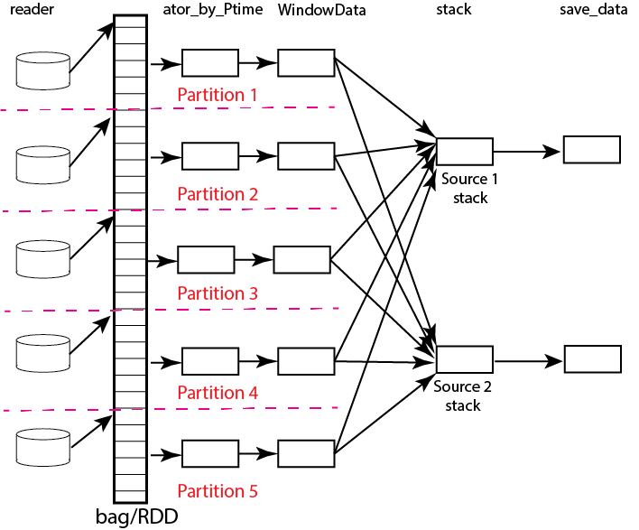
Fig. 20 Data flow diagram for example reduce operation to stack two sources with a bag/rdd made up of atomic TimeSeries data with five partitions. Dashed lines show concept of how partitions divide up the container of data illustrated as a stack of black rectangles. Each rectangle represents a single TimeSeries object. The arrows illustrate data flow from left to right in the figure. As illustrated earlier the reader loads each partition and then makes that data available for processing by other tasks. Processing tasks are illustrated by black rectangles with arrows joining them to other tasks that illustrate the DAG for this workflow. Note that in this case each partition has to be linked to each instance of the stack task. This illustrates why the scheduler has to keep all data in memory before running the stack process as the foldby function has no way of knowing what data is in what partition.#
We emphasize the following that are the lessons you should learn from the above:
The dask foldby method of bag combines two concepts that define the “reduce” operation: (1) a function defining how data to be stacked are grouped, and (2) a function telling dask how the data object are to be combined. The first is the small function we created called keyfunc that returns the value of the source_id. The second is the mspass stack function which will function correctly as a “reduce” operator (For more on that topic see the section titled Parallel Processing.)
In this workflow the left side of the graph is a chain of two map operators like the earlier example in this section. The difference here is the set of pipelines terminate to foci directed at the stack function. That illustrates graphically how the stack function merges multiple inputs into a single output. In this case, it does that by simply summing the inputs to produce one output for each source_id. In terms of memory use this means the final output should normally be much smaller than the inputs.
Our example above shows a best practice that would be normal use for any stack algorithm. That is, the final operator is a call to the save_data method of the database handle (db symbol in this example). The default behavior of save_data is to return only the ObjectId of the inserted waveform document. As a result, on the last line when the compute method is called, dask initiates the calculations and arranges to have the output of save_data returned to the scheduler node. That approach is useful to reduce memory use in the scheduler node and data traffic as calling the output of the compute method is the content of the bag converted to a python list. If the output is known to be small one can change the options of save_data to return the outputs from stack.
Notice that the number of branches on the left side of the DAG is set by the number of partitions in the bag, not the number of objects in the bag. Dask and spark both do this, as noted above, to reduce the size of the DAG the scheduler has to handle.
The biggest potential bottleneck in this workflow is the volume of interprocess communication required between the workers running the ator_by_Ptime and WindowData functions and the stack operator. With a large number of sources a significant fraction of the WindowData outputs may need to be moved to a different node running stack.
The related issue with a foldby operation to that immediately above is the memory requirements. The intermediate step, in this workflow, of creating the bag of stack outputs should, ideally, fit in memory to reduce the chances of significant “spilling” by workers assigned the stack task. The reason is that the grouping function implicit in the above workflow cannot know until the entire input bag is processed where to send all the outputs of the map operations. The stack outputs have to be held somewhere until the left side of the DAG completes.
A final memory issue is the requirements for handling the input. As above the critical, easily set option is the value assigned to the npartitions parameter. We recommend computing the value of \(K_{map}\) with the formula above and setting up the run to assure \(K_{map}<1\). Unless the average number of inputs to stack are small that should normally also guarantee the output of the stack task would not spill.
A second potential form of a “reduce” operation we know of in MsPASS is forming ensembles from a bag of atomic objects. A common example where this will arise is converting TimeSeries data to Seismogram objects. A Seismogram, by definition, is a bundle created by grouping a set of three related component TimeSeries object. The MsPASS bundle function, in fact, requires an input of a TimeSeriesEnsemble. A workflow to do that process would be very similar to the example above using stack, but the stack function would need to be replaced by a specialized function that would assemble a TimeSeriesEnsemble from the outputs of the WindowData function. To do this process one could follow that function by a map operator to run bundle. We have tried that, but found it is a really bad idea. Unless the entire data set is small enough to fit two copies of the data in memory that job can run for very long times from massive spilling or abort on a memory fault. We recommend an ensemble approach utilizing the database to run bundle as described in the next section.
Utilizing Ensembles Effectively#
A large fraction of seismic workflows are properly cast into a framework of processing data grouped into ensembles. Ensemble-based processing, however, is prone to producing exceptional memory use pressure. The reason is simply that the size of the chunks of data the system needs to handle are larger.
Let us first consider a workflow that consists only of a pipeline of map processes like the example above. The memory use can still be quantified by \(K_{map}\) but use the following to compute the nominal data object size:
where \(\bar{N}_{member}\) is the average number of ensemble members, \(\bar {S}_d\) is the average member size, and \(S_{em}\) is the nominal size of each ensemble Metadata container (normally a small factor anyway). Note \(S_d\) is the value \(S_d\) defined above for TimeSeries or Seismogram objects for TimeSeriesEnsemble and SeismogramEnsemble objects respectively. An ensemble-based workflow that terminates in a stacking operation that reduces an ensemble to an atomic data object will have less memory pressure, but is still subject to the same memory pressure quantified by \(K_{map}\).
There is an important class of ensemble processing we noted in the previous section: using the bundle function to create SeismogramEnsemble objects from an input TimeSeriesEnsemble container. Any data originating as miniseed data from an FDSN data center that needs to be handled as three-component data would need to pass through that process. The following is an abbreviated sketch of a standard workflow for that purpose for data logically organized as by source:
#imports would normally be here - omitted for brevity
def make_source_id_queries(db):
  """
  Demonstrates how to generate a list of queries to use as
  input for read_distributed_data to build a bag of ensembles.
  """
  srcidlist = db.wf_miniseed.distinct("source_id")
  querylist = list()
  for id in srcidlist:
    query = {"source_id" : id}
    querylist.append(query)
  return querylist

# Initialization code for database handle (db) would normally be here
matcher = MiniseedMatcher(db)
querylist = make_source_id_queries(db)  # defined above
number_partitions = len(querylist)
mybag = read_distributed_data(querylist,
            db,
            collection="wf_miniseed",
            npartitions=number_partitions,
            )
mybag = mybag.map(detrend)  # not required but more efficiently done at this stage
mybag = mybag.map(normalize,matcher)  # needed to define orientation attributes
mybag = mybag.map(bundle_seed_data)
mybag = mybag.map(db.save_data)
mybag.compute()
This algorithm uses only map operators but can be very memory intensive if the ensembles are large. The reason is that the function bundle_seed_data by necessity has to have two copies of the data in memory; it works through the TimeSeries and assembles the appropriate group of three such objects into Seismogram objects. The example shows the simplest approach to reduce memory use. We create the dask bag with the read_distributed_data function. We pass it the optional parameter npartitions set so each enemble is treated as a single partition. If the ensemble size is large (\(K_{map}<1\)) three approaches can be considered to improve performance.
A common approach is to download data over a longer window than actually needed for a particular study. e.g. one might have an archive of teleseismic event files with miniseed data segments of the order of one hour in length. If the focus is only P waves, windowing with WindowData as used in the earlier example could reduce the data size by an order of magnitude.
Although we’ve never tried this, it should be feasible to create a sequence of MongoDB queries that would sort miniseed data appropriately and group them into smaller bundles of the order of 3 that could be scanned and “bundled” into atomic Seismogram objects with the function
BundleSeedGroup. That workflow would be similar to the one above but the list of queries passed to read_distributed_data would be more complex and usually much larger.If all else fails the workflow can be run as a serial job. For small data sets that can be the best alternative. For very large data sets the time required can be problematic and would only be feasible if the workflow is designed to be restarted from where the last run stopped. For example, the authors ran a benchmark on a desktop system with an extended USArray dataset with all lower 48 station broadband stations in 2013. A job to do the process above alone would have required of the order of weeks on a desktop machine for one year of data. That is a feasible, but awkward calculation by any definition.
There is one final type of ensemble processing worth noting. There are many examples where a logical organization is to read data as atomic data objects, apply some standard tasks like windowing and filtering, and then group the data and assemble them into ensembles for subsequent processing that requires the data to be grouped (e.g. a moment-tensor inversion requires data to be assembled into source-based ensembles.). The problem is that the grouping operation is a form of “reduce/fold” that is can be done efficiently only if the results fit in cluster memory. For that case most will likely find the approach using MongoDB discussed in the next section is superior because it is more readily scaled to arbitrarily large data sets.
Using MongoDB to Manage Memory#
Users should always keep in mind that the ultimate, scalable solution for
memory management is the MongoDB database. If an algorithm applied to
a dataset is memory intensive one question to consider is if there is a
solution using MongoDB? The example immediately above is an example;
running the lower-level BundleSeedGroup could, in principle, be
used to break the problem into smaller chunks. With the right incantation sent to
MongoDB that algorithm is likely a good alternative way to create
Seismogram objects from single station groups of TimeSeries objects.
There are a number of other common algorithms that we know from experience can be handled most easily by utilizing MongoDB.
Any algorithm that requires data to be sorted into a specific order with one or more header (Metadata) attributes is best initiated with MongoDB. There are ways to order a data set in the middle of a workflow, but dask and spark documentation warn that can create a performance issue. Further, assembling the atomic data into ensembles with a function like dask foldby is subject to the memory issues discussed above. Hence, in our experience using MongoDB is a more scalable approach. MongoDB sorting, particularly if used with an appropriate index, is a very efficient way to build a sorted and grouped data set. We should note that ordered data ALWAYS require data to be grouped and loaded into an ensemble container. The reason is that dask and spark do not necessarily preserve order in a map operator. That is, the data in an output bag may be shuffled relative to the input in a map operation. Hence, processing workflows cannot depend on order as is common practice in all seismic reflection processing packages we are aware of.
Dismantling ensembles into atomic components can only be done at present by saving the ensemble data and then reading it back as atomic objects.
As noted in many places in this user’s manual MsPASS uses the idea of a “live” attribute on the native data objects to flag a datum as bad. Such data are carried along in a bag/RDD and consume space because most functions that kill such data leave the data array intact. If a lot of data have been killed, which is common in a major editing step like the snr or edit module functions, memory pressure can often be drastically reduced by removing the dead data. The cleanest way to do that, and preserve the record of what was killed, is to do an intermediate save of the data set and then recreate a new bag/RDD for subsequent processing of the edited data by reading it back again before continuing. In our experience, it is generally useful to treat this as step in processing where the result needs to be reviewed before continuing anyway. The jupyter notebook you create along with records in the database will then preserve your edits.