MsPASS Virtual Cluster Concepts

Audience

This section is mainly for user’s new to MsPASS needing to run the system on an HPC system. Those readers may find the general issue about HPC concepts helpful, but how helpful will be entirely dependent upon the background of the reader. Parts of this section will also be of use to experienced users needing to configure MsPASS for new system. If that is you, then you may find it useful to read this section in combination with the last section of the document titled Deploying MsPASS on an HPC cluster.

All readers should note this section leans heavily on several more specialized sections for specific environments. That is, a primary design goal of MsPASS was scalability. MsPASS is known to allow prototyping a workflow on a desktop system or login node in an HPC system and then porting the same python script with minimal changes to run on a cluster with hundreds of cores. To make that work, however, requires some up-front work to tell the system how to deal with a range of differences that define the system dependencies. An idea we will use repeatedly below is that the configuration process is used to build a virtual cluster.

Finally, for readers new to MsPASS we advise you to consider reading the Introduction section at the same time your read the section here titled Fundamental Concepts. We created these sections to help you understand some of the fundamentals that shaped the design of MsPASS. That background may help you understand material in this document.

Fundamental Concepts

Range of Hardware to run MsPASS

The most basic issue that created a need for a framework like MsPASS is a fundamental change in computing that began more than 20 years ago. That is, prior to that time a computer was synonymous with a single cpu and an associated set of hardware to feed the processor. Today only antique desktops have only one cpu. Multicore processors are now universal other than for specialized hardware like low-power data loggers. The worlds largest “supercomputers” (alias HPC system or cluster) have thousands of nodes and tens of thousands of cores, noting that that sentence is likely to become quickly out of date as the upper limit grows yearly. A special form of computer cluster is what is now called “cloud computing”. Cloud systems add a few special constraints and abstractions, but are fundamentally the same as an HPC cluster in the sense both are a single entry point to a large array of cores. Readers who are unfamiliar with the terminology here of core, multicore, node, multiprocessor, and cloud computing are encouraged to do an internet search on these terms before continuing. The terms encapsulate some key concepts we assume throughout this user manual.

Why is this issue important for seismology? The reason is that all of the most common data analysis tools in our field were developed prior to the multiprocessor revolution. Packages like SAC and the Datascope offline data analysis components of Antelope (Antelope’s real-time system is an exception) are all fundamentally “single-threaded”, which is another way of saying they can only use one cpu in a system at a time. Anyone who has tried to process large data volumes with SAC or Datascope will understand what a severe throttle they impose on what is feasible.

There is one final key point all users must understand about the role of parallel processing versus desktop processing. A concise summary is this: if the processing requires human intervention it probably should not be done on a cluster. That means interactive graphics or any text response within a workflow. The reason, of course, is that human response time to any event is at least 9 orders of magnitude slower than a cpu clock cycle. We thus assume the batch model of processing for HPC and cluster systems wherein a “job” is submitted to a global scheduling system for the cluster. Workflows requiring interactive graphics or other human interaction are normally best run on the HPC login node or move the relevant data to your desktop. Note a key word above is interactive graphics. Workflows that generate saved graphics are required as end products of many workflows and are more than possible through multiple mechanisms. Alternatively, some institutional setups may allow interactive work on your desktop computer accessing the data through a cloud file system, which would have very different performance and use restrictions. A key point is that MsPASS can fill all these roles, but there is a configuration step to run each component in your local computing environment.

Containers

The enabling technology that allows MsPASS to be readily run on a wide variety of platforms is the concept of virtual machine or virtualization. If you are unfamiliar with this topic, an internet search will yield all the sources you can ever have the stomach to read. MsPASS uses a light weight technology than virtual machine called a container. Those who, to use a modern cliche, want to get into the weeds, on this topic may want to read this article

MsPASS currently supports two container technologies:

1. docker is the container software supported by MsPASS. It is the tool of choice for desktop systems. It requires installing a client on your desktop system called, appropriately for this use, docker desktop. The links above contain secondary links to doownload pages and installation instruction for the package.

2. For HPC systems we use a comparable software called singularity. If you are reading this to adapt MsPASS to an HPC system there is probably a web page describing singularity or something similar. If not, there are numerous sources on the web. A simplistic perspective is that singularity is docker for an HPC system. It has command line tools similar to those for docker desktop and runs containers built on docker hub directly. In addition, a fundamental property of singularity is that it runs docker containers directly.

Current cloud systems support docker containers. That is, there is a system dependent procedure to “pull” the MsPASS container but once loaded the container is used directly to run your job.

The key point about containers, in general, is that a container eliminates the long list of system dependency issues that arise with conventional software installation. It also allows MsPASS to run on any operating systems with the x86 architecture (Intel or AMD processors) on the Apple ARM chip used on newer Apple products. Additional hardware support is possible provided docker support it.

Foreman-worker Model

A foundational concept of MsPASS is the foreman-worker model of parallel processing. (Some sources will use the less politically correct term master-slave to describe the came concept.) The idea is simple and intuitive to anyone who has tried to organize a group of people. If you have big job to do that you couldn’t possibly do yourself, you break the job into a set of manageable tasks. The foreman (aka project manager or master) assigns tasks to workers (slaves) as schedule dictates. Dependencies always exist wherein when a worker finishes one task he/she has to pass the result on to another. Three key concepts that appear throughout this user’s manual are direct consequences of this model:

1. The foreman is what we also call a scheduler. That piece of software is the boss whose only job is to assign work.

2. A worker is a single-minded individual who only does what the foreman tells him/her to do (That is why “slave” is sometimes used to describe the concept.).

3. The foreman needs to communicate with the workers to tell them what to do. Less obvious is the fact that all the workers also need to communicate with each other as well as the foreman. The reason is that the most common paradigm is worker A finishes task X and passes the result to to worker B to do task Y where in our case X and Y are two different processing algorithms. As a result interprocesses communication is a fundamental requirement to make processing with the foreman-worker model possible.

Schedulers

As noted a number of other places in this user’s manual MsPASS achieves parallelization in a cluster through one of two schedulers called dask and Spark. Both achieve parallellism by running a series of processes on cores to which the software has access. More details about how these packages do scheduling to achieve parallelism can be found in the links above and a variety of online sources and published books. This section addresses the issue of configuration of MsPASS. For that purpose, you need to understand the following points about setting up dask or spark on a cluster:

1. Most clusters are shared facilities with many simultaneous users. All cluster use some form of higher level scheduler to schedule “jobs”, which is the modern descendant of batch systems developed for “mainframe computers” in the 1960s. A “batch job” means you submit a script of command line instructions to run your application(s) on the system. Hence, the first thing to understand is that to run MsPASS on a cluster will normally require preparing that script of instructions. Part of that script is instructions to the batch scheduler (the software called Slurm in our example below). The batch scheduler has to be told how many nodes and/or cores the job will require and often other resources like minimum memory needs or access to auxiliary resources not required by all jobs. You then “submit” your job script to a “queue”. The batch scheduler then determines when the cluster has sufficient resources available for the time period you define to run your “job”. Do NOT confuse the issue of scheduling a set of nodes for a “job” with the “scheduling” done by Dask/Spark. They are very different things that both utilize the same English word in their definitions.

2. Once a “job” has been scheduled on a cluster task-level scheduling in MsPASS is controlled by dask or Spark. Either require additional configuration setup that tells the software what environment it is running in and how many workers it should define for the job. A less obvious issue with using Spark or Dask is the need to define communication channels between tasks. Both packages use the modern concept of abstracting what “interprocess communication” means. You have no control of what this means for communication between processes running on a single node. In contrast, communication between nodes on HPC systems normally requires some configuration. The reason is that a “job” is assigned a set of nodes (physical machines) by the job scheduler and your script (job) cannot know the network address of those nodes until the job scheduler has assigned them. For that reason we will see below the configuration scripts for HPC setups need a mechanism to ascertain what physical nodes are being used and set up communication channels between them manually.

MongoDB

What MongoDB is, why is chosen for MsPASS, and how it is used in MsPASS are topics discussed throughout this User’s Manual. Two key sections on this topic are Database Concepts and CRUD Operations in MsPASS. The purpose of this section is to clarify several more basic concepts that may help you understand the configuration requirements needed to make MongoDB functional on a cluster.

1. MongoDB like most modern database engines acts in a client-server arrangement. Your application acts as a client and MongoDB is running a service that defines its role as a “server”.

2. Like most servers we have to launch MongoDB as a daemon. That could be done using standard linux methods for launching daemons when the container boots. That approach would not work for MsPASS, however, as when multiple containers are running, which is the norm, the multiple instances would collide. For that reason our setup launches MongoDB manually only on containers defined in the configuration.

3. The MongoDB server communicates with clients through a network connection. As a result a critical configuration parameter is the IP address and port number (If you aren’t familiar with IP numbers and ports there are may internet sources on this topic. This one is a good starting point.) of the node(s) running the MongoDB server.

4. MongoDB has a feature they call sharding. The purpose of sharding is to distribute data on multiple nodes of a cluster to improve performance. The reason that can be a good idea with database intensive operations is database transaction in any database system can be very slow compared to the compute time of the algorithm driving the transactions. That fundamental fact means if your workflow requires extensive database operations that are a bottleneck, sharding is a potential solution. MsPASS supports sharding using MongoDB native setup. That is, turning on sharding is a configuration option.

Frontend

The standard MsPASS container assumes the use of a jupyter notebook to assemble and test your workflow. As noted elsewhere we believe jupyter notebooks are a useful tool to encourage reproducible science. We use a jupyter notebook service to define the role we call frontend. The concept of the frontend is the abstract box that communicates directly with you as the user. The process of driving a jupyter notebook is well documented on many internet pages so if you are not familiar with jupyter notebook we advise you to find a good tutorial on the topic before you try to use MsPASS.

For this overview it is important to stress that the expectation is that you will use jupyter notebook in two ways:

1. Jupyter is an effective tool to assemble and test your python code (your workflow) on a desktop or interactive node in an HPC cluster. The thing jupyter allows that goes far beyond conventional code comments is the ability to insert full-featured text as “markdown” boxes between code blocks. Our tutorials all use this approach and demonstrate this fundamental idea.

2. When you have a functional workflow you want to run on a large cluster to process a full dataset, MsPASS has a feature to run the notebook from the batch job script (see below) using a command line argument.

Perhaps the most important feature of this model is you can and should plan to publish your notebook to allow other scientists to reproduce your work as a near turnkey operation.

MsPASS Configuration

Overview

To understand how to configure MsPASS it is important to first understand some fundamental concepts that are treated as abstractions. You can think of the configuration as making the abstractions concrete.

1. The MsPASS framework is generic and has to be informed about the actual physical configuration. How much it can determine automatically and what it needs to be told manually are system dependent.

2. As much as possible we abstract all IO. That is, Input (I) means you use a handle of some kind to create some data object. Output (O) means you use a handle to save that data in a form that allows it to be reconstructed later. Whether that is done by reading from a file on file system, cloud (via a URL), or something not yet invented is irrelevant. All that matters is that you have a software handle to manage the reads and writes.

3. A special case of IO is interprocess communication. Spark and Dask both abstract that process in a manner opaque to you as a user. This allows them to automatically determine if a connection is process-to-process within a shared memory environment (threads running on the same node) or between nodes. The first is memory-to-memory transfer. For the later it means network communications between two processes on two nodes with the cluster’s internal network.

4. We made a design choice in MsPASS to further abstract the overall system in terms of one of a finite set of functional blocks we refer to as the role. There are four required “roles” any MsPASS setup needs to define: (1) scheduler, (2) worker, db, and frontend. Sharding adds a level of complexity. When sharding is enabled two additional function “roles” are required we call dbmanager (replaces db in a sharded environment) and shard. Finally, we define the role of frontend as an abstraction of the user interface. Sections below will provide more details on what these different “roles” mean and how they are used.

A final point for this overview is that a good summary of the purpose of configuration is to define a virtual cluster in which your job should be run. The scalability of MsPASS is possible because of the abstraction that allows the definition of a virtual cluster. How complicated that configuration will be is dependent upon what you are building. We have a turnkey system for a desktop system, but any other cluster will require a nonzero commitment to configure and run jobs in the virtual cluster you define. MsPASS is a “framework” which means it can handle complex definitions, but it will not produce a workable system until someone adds a skin to the framework.

We first consider a series of example configurations that we illustrate using abstractions we described immediately above. After the examples we turn to the implementation detail of how we make an abstract model concrete.

Example 1: Simple four node virtual cluster

Fig. 2 is a block diagram of a virtual cluster that is largely useful only for it’s pedagogic value. i.e. we show it as an introductory example to help further demonstrate key concepts and how they fit together. The actual configuration here would not be very prudent because it would not make efficient use of resources for reasons we discuss at the end of this section.

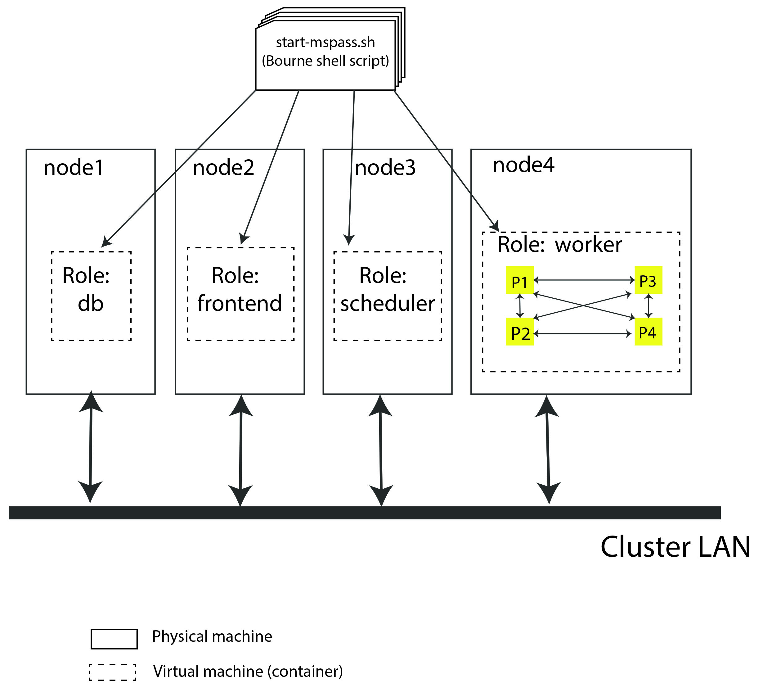
Fig. 2 Block diagram showing abstract components of the virtual cluster configuration of example 1. This example assumes four physical nodes illustrated by the four larger boxes with solid lines. The dashed line boxes define containers running within each physical node. Each physical node is illustrated as connected to a high speed LAN used for node-to-node communication in the cluster.

This simple example is helpful to clarify some important implementation details that we use in MsPASS to define a virtual cluster:

• The functinality of block is driven by what we call a role. In this example shows the four standard roles: db, frontend, scheduler, and worker. Those names define the following:

  • The db container runs MongoDB.

  • The frontend container is running a jupyter notebook service. That is currently the default user interface for MsPASS.

  • The scheduler container runs the dask or spark scheduler.

  • The worker container runs a dask or spark worker.

• This example dedicates each node to a single role and each node runs one instance of the container. We reiterate that would almost certainly be a very inefficient way to build the virtual cluster but is the simplest model one could build.

• When the container is launched it goes through a fast boot process that the setup completes by running the master shell script called start-mspass.sh. start-mspass.sh is a shell script that is part of the container and not something you modify. The script launches different services depending on the role it receives from the launcher (docker or singularity).

• Although in this example we run only one container per physical node, it also shows that the worker node is configured with four processes labeled P1, P2, P3, and P4. Note our terminology has created an ambiguity of language in the current setup you need to understand. A single instance of a container is run with its “role” defined as worker but both dask and spark, by default, will have its worker spin up one process per core defined for that container. That is, a worker hosts multiple processes. That is an important capability of dask and spark as it means all cores of a node can be utilized by a worker.

• The worker node has lines with arrows drawn between the four boxes labeled P1, P2, P3, and P4. Those lines symbolize intra-node, interprocess communication between the worker processes. As noted above dask and spark abstract that communication.

• We illustrate node-to-node communications through a common symbol for a local area network. That is, the heavy line labeled “Cluster LAN”. A key point here is that such communications use a physical connection between nodes and the nodes operating system has to handle routing data traffic to and from the container it is running.

• Fig. 2 has node2 running with a role set as frontend. As noted earlier the frontend box is an abstraction of a user interface but in our implementation it runs the service that allows a web browswer to connect to the virtual cluster by running a jupyter notebook on your local machine. We note that in processing a large data set interactive connections are normally a bad idea and the notebook is normally run in a “batch” mode.

Before continuing it is worth noting why this simple configuration is useful for understanding but likely a bad idea for an actual configuration, The example is useful because of simplicity. In this example each node has one and only one “role”. The examples below show that isn’t essential, but does introduce some potentially confusing complexity we think is important to consider independently. Why this configuration would almost certainly be a “bad idea” for an actual implementation is inefficiency. All but archaic clusters today have multicore nodes. Dedicating a full node to each “role” would waste resources. The most extreme is the frontend box that in our implementation launches a container dedicated only to running a jupyter notebook server. The jupyter notebook server is a very lightweight process that consumes very few resources. Most of the computing in that role is dominated by the python interpreter that for most workflows is lightweight compared to data processing computations. A run in this cofiguration would show node2 nearly idle for an entire run. In contrast, we have found devoting a node to the scheduler role may often be prudent. The key point here is that “fine-tuning” of a production workflow may require some benchmark tests for load balancing. On the other hand, we also caution all users to keep your objectives in mind. If you are doing a one-up workflow for a research project fine-tuning configuration would be a waste of your time. If you face a task with months of compute time, however, some fine-tuning may be justified.

Example 2: Multiple nodes with multiple roles`

Fig. 3 is a block diagram of a virtual cluster that is a minor variant of that in Fig. 2. This configuration has less of the inefficiency of that in Fig. 2 by not dedicating a node to the frontend role. It also illustrates a more subtle point that is an implementation detail we were avoiding in Example 1. That is, note that when a node is set up to run multiple “roles” each role is run in a separate container. We emphasize that is an “implementation detail” we made to simplify the already complicated start-mspass.sh script. We note that approach would have been a bad idea with “virtual machine” software that would require loading a full implmentation of a guest operating system into memory, but this is an example of the merits of a “container”. The approach we used is common and is not at all onerous in the consumption of system resources. The key differences between this and example 1 are:

1. Nodes 1 and 2 are both running two containers with different “roles”.

2. Node 2 illustrates a different configurable feature that can be used to provide better load balancing. That is, it is possible to launch a container running with the role of worker and limit the number of workers that scheduler can assign. This example shows the node 2 worker with only 2 processes while the node dedicated to workers (node 3) is assigned 4 worker processes.

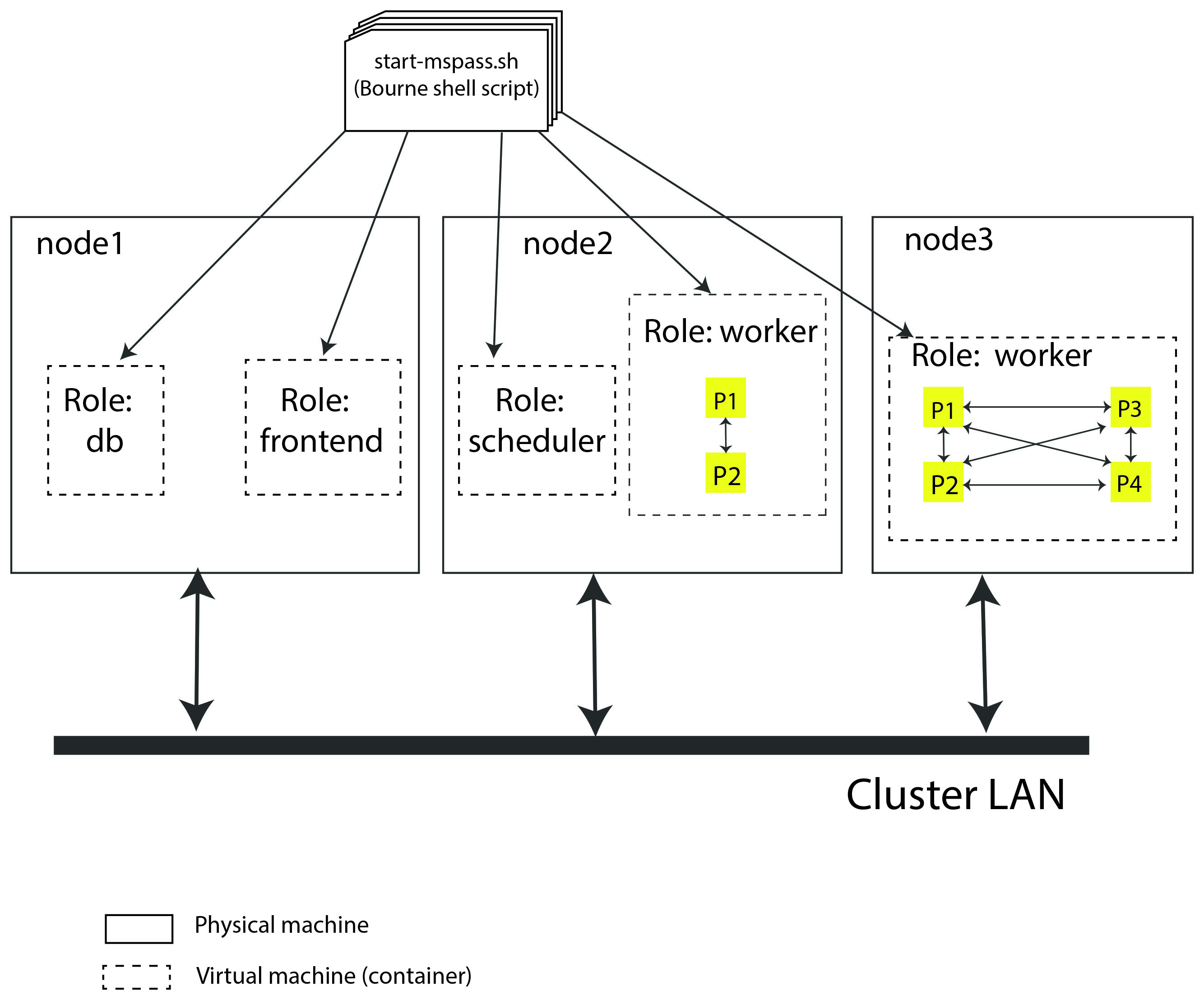
Fig. 3 Block diagram showing abstract components of the virtual cluster configuration of example 2. This example shows a cluster with three physical nodes running containers with multiple roles on two of the three nodes. See the caption of Fig. 2 for details on the meaning of different lines in the diagram.

Example 3: Multiple nodes with optional Sharding

Fig. 4 is the first example that is known to give reasonable load balancing on an HPC system. It is, in fact, a schematic diagram of our example generic configuration for creating a virtual cluster. Configuration files that would create this virtual cluster can be found on github in the directory “scripts/template”. How those scripts are used to define the virtual cluster are described below and in the section of the user manual titled Deploying MsPASS on an HPC cluster

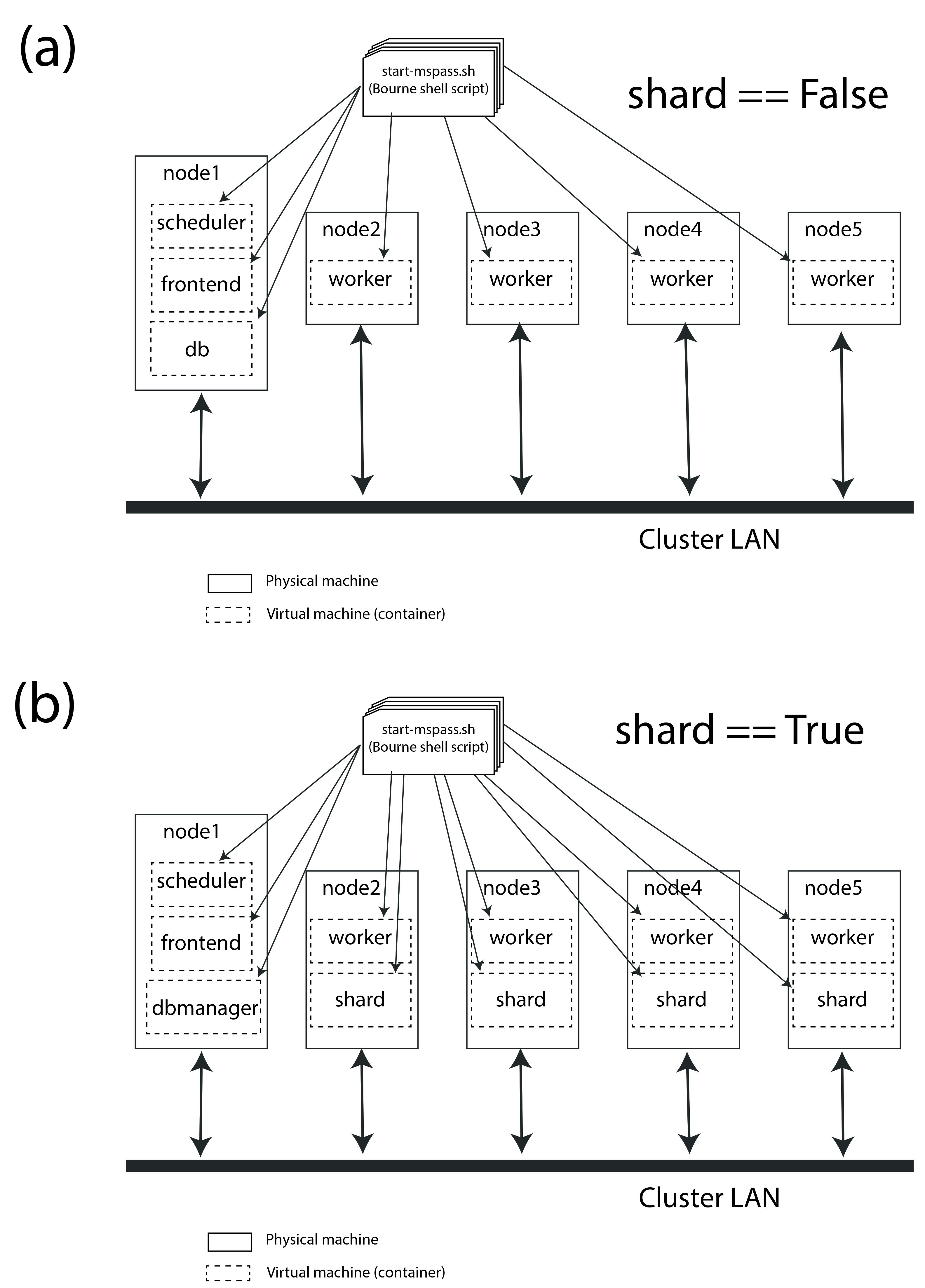
Fig. 4 Block diagram showing abstract components of the virtual cluster configuration of generic templates. This example shows a cluster with five physical nodes. (a) shows a configuration without MongoDB sharding enabled. In that case node 1 has a container running a single instance of MongoDB (box labeled db). Node 1 also has two other containers: one running with role scheduler and another running with role frontend. (b) shows a similar configuration that would be created with the alternative configuration script not enables sharding. Note that in that situation the db box is assigned the role dbmanager. The dbmanager coordinates database transitions with the shards defined in the other nodes. In this example each node running a worker container also runs a container with a role defined as shard.

This figure actually illustrates two different configurations. We consider them together because they are defined by two similar scripts in the scripts/template directory with the file names run_mspass.sh and run_mspas_sharded.sh. How either of these are used in an actual HPC job is discussed below. Here we focus on the abstract configuration they define.

Consider first the case with sharding False (off) as it has much in common with example 2. Some key points about the case with sharding off are the following:

• In this case we have four dedicated worker nodes and put all the other required “roles” in a single node.

• As in example 2 each container runs one and only one role. The worker nodes all run only one container while the node illustrated to the left runs three roles in three different instances of the container.

• We don’t illustrate the worker processes in this figure for simplicity. We note that both dask and spark will default to creating one worker process per core assigned to the container. In this configuration that would normally mean all the cores of that node. Thus if each node had, for example, 16 cores, this virtual cluster would represent a 64 processor engine.

Whether or not this configuration is well balanced depends upon the workflow and the physical nodes on which it is run. Putting the database server on the same node as the scheduler could cause issues for a workflow running lots of database operations.

We show the example with sharding turned on (part b of the figure) as an illustration of how sharding could be enabld to possibly improve load balancing in such a situation with high database traffic. Some key points about the sharding example are the following:

• When sharding is used we add two new MsPASS “role” definitions: shard and dbmanager. We emphasize the “role” concept is a feature of MsPASS and not something you will find in the MongoDB documentation. Both define configurations defined in the start-mspass.sh script used to launch each container. To see exactly what each do look at the contents of start-mspass.sh found here.

• Sharding adds complexity to a setup and run time environment that should not be taken lightly. In general, we would recommend avoiding it unless you have a production workflow you find limited by database transactions.

Example 4: All-in-one desktop setup

We left the special case we call “all-in-one” until now even though virtually all MsPASS users will likely first use it in that mode. The reason is that although it is implemented through the same master script (start-msspas.sh), it is a special case that might be confusing if we had started there. That is, because the framework is primarily designed for running on a cluster running on a desktop has to simulate elements of a cluster. That said, the following figure illustrates an abstraction of the all-in-one mode with symbols the same as the examples above:

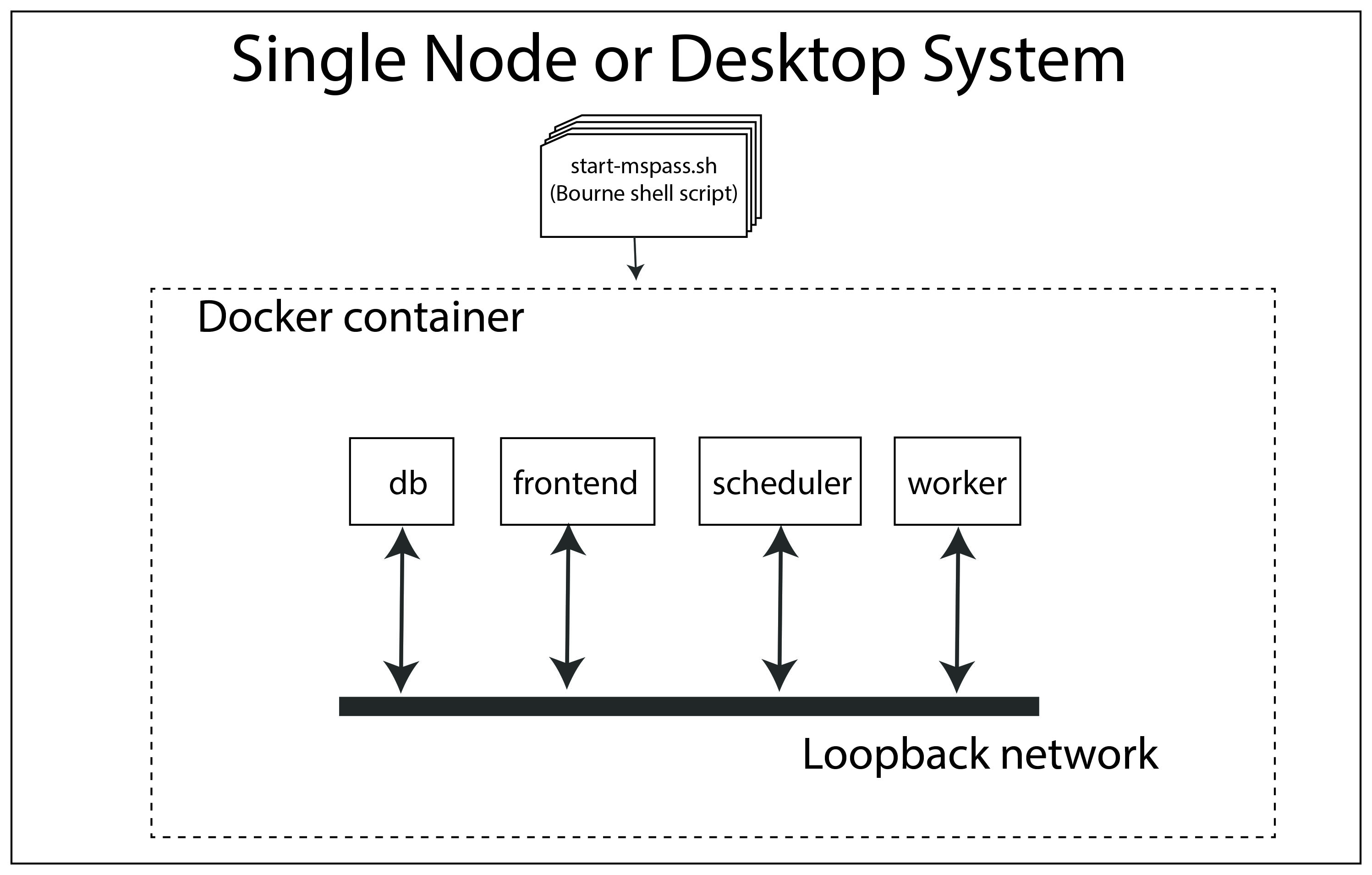
Fig. 5 Block diagram showing abstract components of what we call the all-in-one mode used for running on a single node. Symbols and line styles are as with all the related figures above.

The fundamental difference to note in this run mode is that all four of the required mspass “roles” (scheduler, worker, db, frontend) are run in the same container. All the previous examples used multiple containers with only one “role” per container instance. We emphasize either choice (one role per container or multiple roles per container instance) is an implementation detail. The single container mode is more straightforward for a desktop. Multiple containers are more appropriate for clusters to make the configuration more generic. When you see docker/singularity containers as being “lightweight” part of what that means is that multiple instances can be run on the same node with minimal performance impact.

A final point about this configuration is that by default both dask and spark will define the number of process devoted to workers to be the number of cores defined for the container. If you are running MsPASS on a desktop you want to simultaneously use for other purposes you may want to configure docker to not use all the cores on the system. That process is described here.

HPC Job Submission

A final point anyone running MsPASS on an HPC cluster needs to understand is how a “job” (aka your workflow) is run on such a cluster. We first consider how a batch job is run since most HPC compute jobs should be run that way. Fig. 6 is a graphic that we use as an aid to explaining the process.

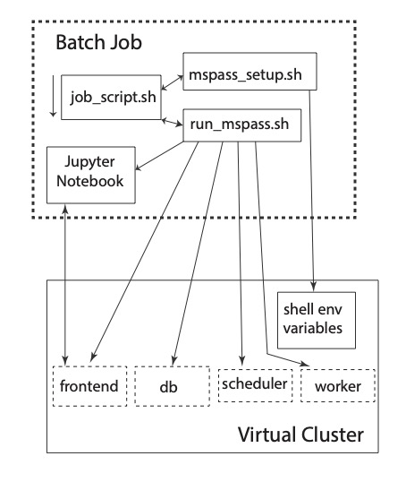
Fig. 6 Block diagram illustrating how jobs are run on an HPC system with MsPASS. Main text uses this figure for a detailed description of the process.

There are two large boxes in that figure. The box defined by a heavy dashed line box and labeled “Batch Job” encloses a set of four smaller boxes that represent four files that define a particular “job”. Three are unix shell scripts that contains unix shell commands that are executed sequentially on the native operating system of one or more of the physical nodes. The fact that there are three files for this process is an implementation detail in our setup done to make it easier for an individual user to create and run jobs. Details of how these files are customized for a particular setup are given in Deploying MsPASS on an HPC cluster. For the present you should understand that the box labeled job_script.sh in the figure is the shell script you submit to the cluster scheduler (slurm or the equivalent). It acts like “main” in a C/FORTRAN program. The two auxiliary files illustrated as boxes in the figure and labeled mspass_setup.sh and run_mspass.sh act like functions/subroutines where they execute to completion and return control to job_script.sh. mspass_setup.sh is used only to put all the user-specific setup parameters in a single place. In standard unix shell fashion that is done with “environment variables”. As the figure illustrates you can think of that process as setting environment variables in the run area of the virtual cluster.

The second subroutine-like shell script, which is labeled as run_mspass.sh in the figure, is more complex but is static for a particular cluster. That is, many jobs can run with the same run_mspass.sh setup. It is the recipe for defining a partiular configuration for the “virtual cluster”. The main thing that shell script does is launch the set of one or more container defining the four required “roles” that together define a particular virtual cluster setup. That is illustrated in the figure with the boxes with dashed lines enclosing the four role keywords. The fact those functional boxes are launched by run_mspass.sh is illustrated by the arrows running from the box for the script and each of the dashed line boxes in the virtual cluster with a particular role. Each of the launching steps use one or more environment variables to define key setup parameters. Note the reason no containers instances are illustrated within the virtual cluster box is that from the job script’s perspective that is an implementaton detail. The perspective you should have when writing any variation of job_script.sh is that run_mspass.sh creates the virtual cluster. Note also we illustrate one worker in the figure only to keep the figure simple. The virtual cluster box is open-ended and could conceivably define hundreds of workers.

The final file that drives the processing is the box with the tag “Jupyter Notebook”. The last line of the run_mspass.sh script launches the jupyter notebook server in a mode where the server immediately loads and executes a notebook file you specify as an argument to job_script.sh. The entire job terminates when the notebook finishes (or exits on an error). The line launching the jupyter notebook server (“frontend” role) blocks until the notebook server exits. Control is then returned to job_script.sh which either does cleanup or exits. The cluster management software (slurm or the equivalent) then kills all the running containers. Fig. 7 is a similar to Fig. 6 but illustrates how a “job” is run on an HPC virtual cluster if you need to run a notebook interactively.

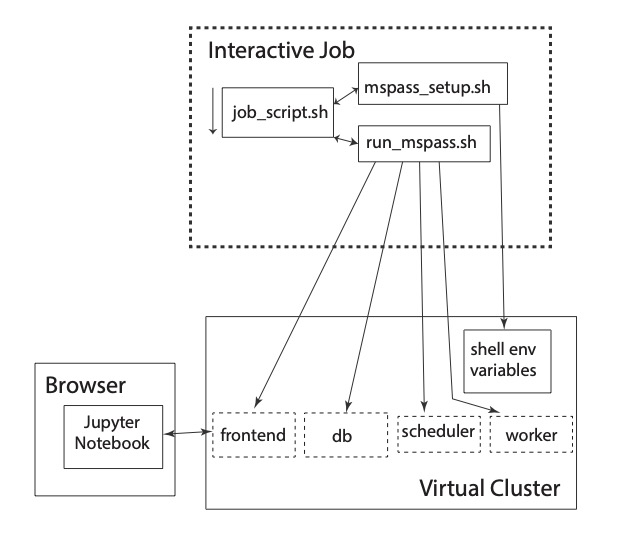
Fig. 7 Block diagram illustrating how jobs are run on an HPC system with MsPASS when human interaction with the jupyter notebook server is required.

A comparison of the two figures may be helpful. The only difference is in this case we show a connection to the “frontend” box from a web browser illustrated as box on the left hand side of the figure. The actual run procedure has only one difference; when the jupyter notebook server is launched it doesn’t immediately start executing a script but waits on input from the user. Hence, when you run a notebook one code box at a time, which is the typical interactive use, the virtual cluster only does computing when each box is run. With that understanding it should be clear that running a job in this mode is a really bad idea unless you are forced to do so to debug a problem. The smallest human response time is many orders of magnitude slower than any of the processors. On HPC when your job is running you are the only user on the nodes reserved for your job. Needless to say running a large job in interactive mode can be a serious waste of resources. For that reason the standard approach you should use is to develop any workflow is a three step procedure:

1. Develop the notebook workflow on a desktop system with a small subset of the larger data set you aim to process.

2. Transfer the (working) notebook and test file to the HPC system. Run it in batch mode and verify it gives the same answer.

3. Submit the workflow to the HPC system with modifications to process the full data set.

There is one final variant worth noting that is not illustrated in either Fig. 6 or Fig. 7. That is, dask has a useful diagnostic dashboard that can be used for real-time monitoring of a job. The reason is that graphically the setup is identical to that illustrated in Fig. 7. The difference is that the job would normally still be run in batch mode, but the external web browser would connect to the “diagnostic port” (8787 by default) instead of the network port used by the notebook server (normally 8888). We note that any variation of Fig. 7 an external web browser will only be able to make such a connection if networking to the cluster is set up to allow that connection. We discuss those issues and potential solution in the related section titled Deploying MsPASS on an HPC cluster.