Data Object Design Concepts

Overview

The core data objects in MsPASS were designed to encapsulate the most atomic objects in seismology waveform processing: scalar (i.e. single channel) signals, and three-component signals. The versions of these you as a user should normally interact with are two objects defined in MsPASS as TimeSeries and Seismogram respectively.

These data objects were designed to simply interactions with MongoDB. MongoDB is completely flexible in attribute names handled by the database. In all cases, the components of a data object should be conceptualized as four distinct components handled separately and discussed in more detail below:

The waveform data (normally the largest in size).
A generalization of the traditional concept of a trace header. These are accessible as simple name value pairs but the value can be anything. It is a bit like a python dictionary, but implemented with standard C++.
An error logger that provides a generic mechanism to post error messages in a parallel processing environment.
An optional object-level processing history mechanism.

Data objects are grouped in memory with a generic concept called an Ensemble. The implementation in C++ uses a template to define a generic ensemble. A limitation of the current capability to link C++ binary code with python is that templates do not translate directly. Consequently, the python interface uses two different names to define Ensembles of TimeSeries and Seismogram objects: TimeSeriesEnsemble and SeismogramEnsemble respectively.

The C++ objects have wrappers for python that hide implementation details from the user. All MongoDB operations implemented with the pymongo package use these wrappers. Compute intensive numerical operations on the sample data should either be written in C/C++ with their own wrappers or exploit numpy/scipy numerical routines. The later is possible because the wrappers make the data arrays look like numpy arrays.

History

It might be helpful for the user to recognize that the core data objects in MsPASS are the second generation of a set of data objects developed by one of the authors (Pavlis) over a period of more than 15 years. The original implementation was developed as a component of Antelope. It was distributed via the open source additions to Antelope distributed through the Antelope user’s group and referred to as SEISPP. The bulk of the original code can be found here in github, and doxygen generated pages comparable to those found with this package can be found here.

To design the core data objects from this older library we followed standard advice and mostly burned the original code keeping only the most generic components needed to handle concepts the authors had found essential over the years. The revisions followed these guidelines:

Make the API as generic as possible.
Use inheritance more effectively to make the class structure more easily extended to encapsulate different variations in seismic data.
Divorce the API completely from Antelope to achieve the full open source goals of MsPASS. Although not implemented at this time, the design will allow a version 2 of SEISPP in Antelope, although that is a “small matter of programming” that may never happen.
Eliminate unnecessary/extraneous constructors and methods developed by the authors as the class structure evolved organically over the years. In short, think through the core concepts more carefully and treat SEISPP as a prototype.
Extend the Metadata object (see below) to provide support for more types (objects) than the lowest common denominator of floats, ints, strings, and booleans handled by SEISPP.
Reduce the number of public attributes to make the code less prone to user errors. Note the word “reduce” not “eliminate” as many books advise. The general rule is simple parameter type attributes are only accessible through getters and putters while the normally larger main data components are public. That was done to improve performance and allow things like numpy operations on data vectors.

MsPASS has hooks to and leans heavily on obspy. We chose, however, to diverge some from obspy in some fundamental ways. We found two fundamental flaws in obspy for large scale processing that required this divergence:

obspy handles what we call Metadata through set of python objects that have to be maintained separately and we think unnecessarily complicate the API. We aimed instead to simplify the management of Metadata as much as possible. Our goal was to make the system more like seismic reflection processing systems that manage the same problem through a simple namespace wherein metadata can be fetched with simple keys. We aimed to hide any hierarchic structures (e.g relational database table relationships, obspy object hierarchies, or MongoDB normalized data structures) behind the (python) Schema object to reduce all Metadata to pure name:value pairs.
obspy does not handle three component data in a native way, but mixes up the concepts we call Seismogram and Ensemble in to a common python object they define as a Stream. We would argue our model is a more logical encapsulation of the concepts that define these ideas. For example, a collection of single component data like a seismic reflection shot gather is a very different thing than a set of three component channels that define the output of three sensors at a common point in space. Hence, we carefully separate TimeSeries and Seismogram (our name for Three-Component data). We further distinguish Ensembles of each atomic type.

Core Concepts

Overview - Inheritance Relationships

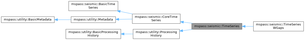
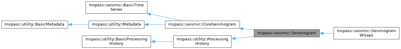
The reader needs to first see the big picture of how TimeSeries and Seismogram objects are defined to understand the core concepts described in sections that follow. We assume the reader has some understanding of the concepts of inheritance in object oriented code. The inheritance structure is best understood as derived from the SEISPP prototype (see history above). We aimed to rebranch and prune SEISPP based on the experience from 15 years of development for SEISPP.

The (admittedly) complicated inheritance diagrams for TimeSeries and Seismogram objects generated by doxygen are illustrated below

Notice that both CoreSeismogram and CoreTime series have a common inheritance from three base classes: BasicTimeSeries, BasicMetadata, and BasicProcessingHistory. Python supports multiple inheritance and the wrappers make dynamic casting within the hierarchy (mostly) automatic. e.g. a Seismogram object can be passed directly to a python function that does only Metadata operations and it will be handled seamlessly because python does not enforce type signatures on functions. CoreTimeSeries and CoreSeismogram should be thought of a defining core concepts independent from MsPASS. All MsPASS specific components are inherited from ProcessingHistory. ProcessingHistory implements two important concepts that were a design goal of MsPASS: (a) a mechanism to preserve the processing history of a piece of data to facilitate more reproducible science results, and (b) a parallel safe error logging mechanism. A key point of the design of this class hierarchy is that future users could chose to prune the ProcessingHistory component and reuse CoreTimeSeries and CoreSeismogram to build a completely different framework.

We emphasize here that users should normally expect to only interact with the TimeSeries and Seismogram objects. The lower levels sometimes but not always have python bindings.

The remainder of this section discusses the individual components in the class hierarchy.

BasicTimeSeries - Base class of common data characteristics

This base class object can be best viewed as an answer to this questions: What is a time series? Our design answers this question by saying all time series data have the following elements:

We define a time series as data that has a fixed sample rate. Some people extend this definiion to arbitrary x-y data, but we view that as wrong. Standard textbooks on signal processing focus exclusively on uniformly sampled data. With that assumption the time of any sample is virtual and does not need to be stored. Hence, the base object has methods to convert sample numbers to time and the inverse (time to sample number).
Data processing always requires the time series have a finite length. Hence, our definition of a time series directly supports windowed data of a specific length. The getter for this attribute is npts() and the setter is set_npts(int). This definition does not preclude an extension to modern continuous data sets that are too large to fit in memory, but that is an extension we don’t currently support.
We assume the data has been cleaned and lacks data gaps. Real continuous data today nearly always have gaps at a range of scale created by a range of possible problems that create gaps: telemetry gaps, power failures, instrument failures, time tears, and with older instruments data gaps created by station servicing. MsPASS has stub API definitions for data with gaps, but these are currently not implemented. Since the main goal of MsPASS is to provide a framework for efficient processing of large data sets, we pass the job of finding and/or fixing data gaps to other packages or algorithms using MsPASS with a “when in doubt throw it out” approach to editing. The machinery to handle gap processing exists in both obpsy and Antelope and provide possible path to solution for users needing more extensive gap processing functionality.

BasicTimeSeries has seven internal attributes that are accessible via getters and (when absolutely necessary) can be set by the user with setters. Most are best understood from the class documentation, but one is worth highlighting here. A concept we borrowed from seismic reflection is the idea of marking data dead or alive; a boolean concept. There are methods to ask if the data are alive or dead (live() and dead() respectively) and setters to force live (set_live()) or dead (kill()). An important thing to note is that an algorithm should always test if a data object is defined as live. Some algorithms may choose to simply pass data marked dead along without changing or removing it from the workflow. Failure to test for the live condition can cause mysterious aborts when an algorithm attempts to process invalid data.

Handling Time

MsPASS uses a generalization to handle time that is the same as a novel method used in the original SEISPP library. The concept can be thought of as a generalized, but yet simplified version of how SAC handles time. The time standard is defined by an enum class in C++ called tref which is mapped to fixed names in python. There are currently two options:

When tref is TimeReferenceType::Relative (TimeReferenceType.Relative in python) the computed times are some relatively small number from some well defined time mark. The most common relative standard is the implicit time standard used in all seismic reflection data: shot time. SAC users will recognize this idea as the case when IZTYPE==IO. Another important one used in MsPASS is an arrival time reference, which is a generalization of the case in SAC with IZTYPE==IA or ITn. We intentionally do not limit what this standard actually defines as how the data are handled depends only on the choice of UTC versus Relative. The ASSUMPTION is that if an algorithm needs to know the answer to the question, “Relative to what?”, that detail will be defined in a Metadata attribute.
When tref is TimeReferenceType::UTC (TimeReferenceType.UTC in python) all times are assumed to be an absolute time standard defined by coordinated universal time (UTC). We follow the approach used in Antelope and store ALL times defined as UTC with unix epoch times. We use this simple approach for two reasons: (1) storage (times can be stored as a simple double precision (64 bit float) field), and (2) efficiency (computing relative times is trivial compared to handling calendar data). This is in contrast to obspy which require ALL start times (t0 in mspass data objects) be defined by a python class they call UTCDateTime. Since MsPASS is linked to obspy we recommend you use the UTCDateTime class in python if you need to convert from epoch times to one of the calendar structures UTCDateTime can handle.

A more concise summary of what these two time standard mean is this: active source data always use Relative time and earthquake data are always stored in raw form as UTC time stamps (e.g. see the SEED standard). UTC is a fixed standard while Relative could have other meanings.

The enum class syntax to define tref is awkward at best. Consequently, we provide two convenience methods that have been wrapped for use in python as as well as C++ code: (a) time_is_relative() returns true if the time base is relative, and (b) time_is_UTC() returns true if the time standard is UTC.

BasicTimeSeries defines two methods to convert between these two time standards: rtoa (Relative to Absolute) and ator (Absolute to Relative). Be aware the library has internal checks to avoid an invalid conversion from relative to absolute with the rtoa() method. This was done to avoid errors from trying to convert active source data to an absolute time standard when the true time is not well constrained.

For an expanded discussion on this topic go here.

Metadata Concepts

All data objects used by the MsPASS C++ library inherit a Metadata object. A Metadata object is best thought of through either of two concepts well known to most seismologists: (1) headers (SAC), and (2) a dictionary container in python. Both are ways to handle a general, modern concept of metadata commonly defined as “data that provides information about data”. Packages like SAC use fixed (usually binary fields) slots in an external data format to define a finite set of attributes with a fixed namespace. obspy uses a python dictionary like container they call Stats to store comparable information. That approach allows metadata attributes to be extracted from a flexible container addressable by a key word and that can contain any valid data. For example, a typical obspy script will contain a line like the following to fetch the station name from a Trace object d.

sta=d.Stats["station"]

In MsPASS we use a similar concept based on Pavlis’s SEISPP library but developed a number of years before obspy. The Metadata object in MsPASS, however, has additional features not in the older SEISPP version.

The mspass::Metadata object has a container that can hold any valid data much like a python dictionary. The current implementation uses the any library that is part of the widely used boost library. In a C++ program Metadata can contain any data that, to quote the documentation from boost, is “copy constructable”. Thus Metadata acts much like a python dict using put and get operations within a python program.

The flexibility of either a python dict or Metadata present a serious potential for unexpected results or crashes if not managed. Any algorithm implemented in a lower level language like C/C++ or FORTRAN and exposed to python through wrappers is subject to crashing from type collisions. The fundamental problem is that python is relatively cavalier about type while both C/C++ and FORTRAN are “strongly typed”. MongoDB storage of attributes can be treated as dogmatic or agnostic about type depending on what language API is used. In MsPASS all database operations are currently done through python, so Metadata or python dict data can be saved and restored seamlessly with little concern about enforcing the type of an attribute. Problems arise when data loaded as Metadata from MongoDB are passed to algorithms that demand an attribute have a particular type that is not, in fact, the type python guessed or received from storage in MongoDB. Consider this example:

d={'time':10}
type(d['time'])

The interpreter will respond to the second line with: <class ‘int’>. If a program wanted to use the time attribute and expected a real number it may crash or produce unexpected results.

In designing MsPASS we were faced with how to cleanly manage this mismatch in language behavior without being too heavy handed and end up making a framework that was too ponderous to use? Our design sets these requirements:

Within an individual application managing the namespace of attributes and type associations should be as flexible as possible to facilitate adapting legacy code to MsPASS. We provide a flexible aliasing method to map between attribute namespaces to make this possible. Any such application, however, must exercise care in any alias mapping to avoid type mismatch. We expect such mapping would normally be done in python wrappers.
Attributes stored in the database should have predictable types whenever possible. We use a python class called Schema described below to manage the attribute namespace is a way that is not especially heavy handed. Details are given below when we discuss the database readers and writers.
Care with type is most important in interactions with C/C++ and FORTRAN implementations. Pure python code can be pretty loose on type at the cost of efficiency. Python is thus the language of choice for working out a prototype, but when bottlenecks are found key sections may need to be implemented in a compiled language. In that case, the Schema rules provide a sanity check to reduce the odds of problems with type mismatches.

The MsPASS C++ api for Metadata has methods that are dogmatic about type and methods that can take anything. Core support is provided for types supported by all database engines: real numbers (float or double), integers (32 or 64 bit), strings (currently assumed to be UTF-8), and booleans. These functions are dogmatic and strongly enforce type throwing a MsPASSError exception if there is a mismatch.

There are four strongly-typed “getters” seen in the following contrived code segment:

# Assume d is a Seismogram or TimeSeries which automatically casts to a Metadata in the python API use here
x=d.get_double("t0_shift")   # example fetching a floating point number - here a time shift
n=d.get_int("evid")   # example feching integer - here an event id
s=d.get_string("sta")  # example fetching a UTF-8 string
b=d.get_bool("LPSPOL") # boolean for positive polarity used in SAC

There are comparable, strongly-typed “putters”:

d.put_double("t0_shift",x)
d.put_int("evid",n)
d.put_string("sta",s)
d.put_bool("LPSPOL",True)

A more flexible although potentially more dangerous element of the API are generic getters and setters that will take any valid python object. For example, if the variable “name_list” below was a python list of something like seismic station names one can use this construct:

d.put("names",name_list)
# or using a decorator defined in MsPASS
d["names"]=name_list

We can then retrieve that list with the inverse

x=d.get("names")
# or using a decorator defined in MsPASS
x=d["names"]

A basic rule is to use the strongly typed API for attributes needed by algorithms implemented in compiled languages and use generic object attributes with care.

An important footnote to this section is that a mspass::utility::Metadata object can be constructed directly from a python dict. That is used, for example, in MongoDB database readers because a MongoDB “document” is returned as a python dict in MongoDB’s python API.

Managing Metadata type with mspasspy.db.Schema

Most type enforcement is imposed by data readers and writers where the Schema class is automatically loaded with the Database class that acts as a handle to interact with MongoDB. Here we only document methods available in the Schema class and discuss how these can be used in developing a workflow with MsPASS.

The most important implementation of Schema is a subclass with the name MetadataSchema. You can create an instance easily like this:

from mspasspy.db.schema import MetadataSchema
 schema=MetadataSchema()

MetadataSchema currently has two main definitions that can be extracted from the class as follows:

mdseis=schema.Seismogram
 mdts=schema.TimeSeries

There are minor variations in the namespace between these two definitions, but the restrictions they impose can be interogated through a common interface. Both the mdseis and mdts symbols above are instances of a the MDSchemaDefinition class described here.

The key point for this introduction is that the mdseis and mdts objects contain methods that can be used to get a list of restricted symbols (the keys() method), the type that the framework expects that symbol to define (the type() method), and a set of other utility methods.

One subset of the methods of the MDSchemaDefinitions class that deserves particular discussion is a set of methods designed to handle aliases. These methods exist to simplify the support in the framework for adapting other packages that use a different set of names to define a common concept. For example, although at this writing we haven’t attempted this the design was intended to support things like automatic mapping of MsPASS names to and from SAC header names. We expect similar capabilities should be make it feasible to map CSS3.0 attributes (e.g. Antelope’s Datascope database implementation uses the CSS3.0 schema) loaded from relational database joins directly into the MsPASS namespace. The methods used to handle aliases are readily apparent from the documentation page linked above as they all contain the keyword alias. We leave the exercise of understanding how to use this feature to planned tutorials.

Scalar versus 3C data

MsPASS currently supports two different atomic data objects: TimeSeries objects are used to store single channel data while Seismogram objects are used to store data from three component instruments. TimeSeries objects are based on the standard concept for storing scalar data that has been around since the earliest days of digital seismic data in the oil and gas industry. That is, the sample values are stored in a continuous block of memory that can be treated mathematically as a vector. The index for the vector serves as a proxy for time (the time method in BasicTimeSeries can be used to convert an index to a time defined as a double). Note in mspass the integer index always uses the C convention starting at 0 and not 1 as in FORTRAN, linear algebra, and many signal processing books. We use a C++ standard template library vector container to hold the sample data accessible through the public variable s in the C++ api. The python API makes the vector container look like a numpy array that can be accessed in same way sample data are handled in an obspy Trace object in the “data” array. It is important to note that the C++ s vector is mapped to data in the python API. The direct interface through numpy/scipy allows one to manipulate sample data with numpy or scipy functions (e.g. simple bandpass filters). That can be useful for testing and prototyping but converting and algorithm to a parallel form requires additional steps described here (LINK to parallel section)

Although scalar time series data are treated the same (i.e. as a vector) in every seismic processing system we are aware of, the handling of three component data is not at all standardized. There are several reasons for this created by some practical data issues:

Most modern seismic reflection systems provide some support for three-component data. In reflection processing scalar, multichannel raw data are often treated conceptually as a matrix with one array dimension defining the time variable and the other index defined by the channel number. When three component data are recorded the component orientation can be defined implicitly by a component index number. A 3C shot gather than can be indexed conveniently with three array indexes. A complication in that approach is that which index is used for which of the three concept required for a gather of 3C data is not standarized. Furthermore, for a generic system like mspass the multichannel model does not map cleanly into passive array data because a collection of 3C seismograms may have irregular size, may have variable sample rates, and may come from variable instrumentation. Hence, a simple matrix or array model would be very limiting and is known to create some cumbersome constructs.
Traditional multichannel data processing emerged from a world were instruments used synchronous time sampling. Seismic reflection processing always assumes during processing that time computed from sample numbers is accurate to within one sample. Furthermore, the stock assumption is that all data have sample 0 at shot time. That assumption is a necessary condition for the conceptual model of a matrix as a mathematical representation of scalar, multichannel data to be valid. That assumption is not necessarily true (in fact it is extremely restrictive if is required) in passive array data and raw processing requires efforts to make sure the time of all samples can be computed accurately and time aligned. Alignment for a single station is normally automatic although some instruments have measurable, constant phase lags at the single sample level. The bigger issue for all modern data is that the raw data are rarely stored in a multiplexed multichannel format, although the SEED format allows that. Most passive array data streams have multiple channels stored as compressed miniSEED packets that have to be unpacked and inserted into something like a vector container to be handled easily by a processing program. The process becomes more complicated for three-component data because at least three channels have to be manipulated and time aligned. The obspy package handles this issue by defining a Stream object that is a container of single channel Trace objects. They handle three component data as Stream objects with exactly three members in the container.

We handle three component data in MsPASS by using a matrix to store the data for a given Seismogram. The data are directly accessible in C++ through a public variable called u that is mnemonic for the standard symbol used in the old testament of seismology by Aki and Richards. In python we use the symbol data for consistency with TimeSeries. There are two choices of the order of indices for this matrix. The MsPASS implementation makes this choice: a Seismogram defines index 0(1) as the channel number and index 1(2) as the time index. The following python code section illustrates this more clearly than any words:

from mspasspy.ccore.seismic import Seismogram
d = Seismogram(100)  # Create an empty Seismogram with storage for 100 time steps initialized to all zeros
d.data[0,50] = 1.0   # Create a delta function at time t0+dt*50 in component 0

Note as with scalar data we use the C (and python) convention for indexing starting at 0. In the C++ API the matrix is defined with a lightweight implementation of a matrix as the data object. That detail is largely irrelevant to python programmers as the matrix is made to act like a numpy matrix by the wrappers. Hence, python programmers familiar with numpy can manipulate the data matrix with all the tools of numpy noting that the data are in what numpy calls FORTRAN order.

The Seismogram object has a minimal set of methods that the authors consider core concepts defining a three component seismogram. We limit these to coordinate transformations of the components. There are multiple methods for rotation of the components (overloaded rotate method), restoring data to cardinal directions at the instrument (rotate_to_standard), Kennett’s free surface transformation, and a general transformation matrix. We use a pair of (public) boolean variables that are helpful for efficiency: components_are_orthogonal is true after any sequence of orthogonal transformations and components_are_cardinal is true when the components are in the standard ENZ directions.

The process of creating a Seismogram from a set of TimeSeries objects in a robust way is not trivial. Real data issues create a great deal of complexity to that conversion process. Issues include: (a) data with a bad channel that have to be discarded, (b) stations with multiple sensors that have to be sorted out, (c) stations with multiple sample rates (nearly universal with modern data) that cannot be merged, (d) data gaps that render one or more components of the set incomplete, and (e) others we haven’t remembered or which will appear with some future instrumentation. To handle this problem we have a module in MsPASS called bundle documented here(THIS NEEDS A LINK - wrote this when bundle had not yet been merged).

Ensembles of TimeSeries and Seismogram data are handled internally with a more elaborate C++ standard template library container. For readers familiar with C++ the generic definition of an Ensemble is the following class definition created by stripping the comments from the definition in Ensemble.h):

template <typename Tdata> class Ensemble : public Metadata
{
public:
  vector<Tdata> member;
  // ...
  Tdata& operator[](const int n) const
  // ...
}

where we omit all standard constuctors and methods to focus on the key issues here. First, an Ensemble should be thought of as a vector of data objects with a Metadata object to store attributes common to the entire ensemble. Hence, the idea is to store global attributes in the Ensemble Metadata field. The vector container makes it simple to handle an entire group (Ensemble) with a simple loop. e.g. here is a simple loop to work through an entire Ensemble (defined in this code segment with the symbol d) in order of the vector index:

n=d.member.size()
for i in range(n):
  somefunction(d.member[i])    # pass member i to somefunction

The wrappers also make the ensemble members “iterable”. Hence the above block could also be written:

for x in d.member:
  somefunction(x)

ProcessingHistory and Error Logging

Core versus Top-level Data Objects

The class hierarchy diagrams above illustrate the relationship of what we call CoreTimeSeries and CoreSeismogram objects to those we call TimeSeries and Seismogram respectively. That design was aimed to make the Core objects more readily extendible to other uses than MsPASS. We encourage users to consider using the core objects as base classes for other ways of handling any kind of time series data that match the concepts defined above.

The primary distinction between CoreTimeSeries and CoreSeismogram and their higher level representation as TimeSeries and Seismogram is the addition of two additional classes that implement two different fundamental, but auxiliar concepts: (1) processing history and (2) error logging. The motivation for these two concepts was discussed above. Here we focus on the data structure they impose. Other sections expand on the details of both classes.

Both TimeSeries and Seismogram objects extend their “core” parents by adding two classes:

ProcessingHistory, as the name implies, can (optionally) store the a complete record of the chain of processing steps applied to a data object to put it in it’s current state. The complete history has two completely different components described in more detail elsewhere in this User’s Manual: (a) global job information designed to allow extracting the full instance of the job stream under which a given data object was produced, and (b) a chain of parent waveforms and algorithms that modified them to get the data in the current state. Maintaining processing history is a complicated process that can lead to memory bloat in complex processing if not managed carefully. For this reason this feature is off by default. Our design objective was to treat object level history as a final step to create a reproducible final product. That would be most appropriate for published data to provide a mechanism for others to reproduce your work, archival data to allow you or others in your group to start up where you left off, or just for a temporary archive to preserve what you did.
ErrorLogger is an error logging object. The purpose of the error logger is to maintain a log of any errors or informative messages created during the processing of the data. All processing modules in MsPASS are designed with global error handlers so that they should never abort, but in worst case post a log message that tags a fatal error. (Note if any properly structured mspass enabled processing function throws an exception and aborts it has encountered a bug that needs to b reported to the authors.) In our design we considered making the ErrorLogger a base class for Seismogram and TimeSeries, but it does not satisfy the basic rule of making a concept a base class if the child “is a” ErrorLogger. It does, however, perfectly satisfy the idea that the object “has an” ErrorLogger. Both TimeSeries and Seismogram use the symbol elog as the name for the ErrorLogger object (e.g. If d is a Seismogram object, d.elog, would refer to the error logger component of d.)’’

Object Level History Design Concepts

As summarized above the concept we wanted to capture in the history mechanism was a means to preserve the chain of processing events that were applied to get a piece of data in a current state. Our design assumes the history can be described by an inverted tree structure. That is, most workflows would merge many pieces of data (a reduce operation in map-reduce) to produce a given output. The process chain could then be viewed as tree growth with time running backward. The leaves are the data sources. Each growth season is one processing stage. As time moves forward the tree shrinks from many branches to a single trunk that is the current data state. The structure we use, however, is more flexible than real tree growth. Many-to-many mixes of data will produce a tree that does not look at all like the plant forms of nature, but we hope the notion of growth seasons, branch, and trees is useful to help understand how this works.

To reconstruct the steps applied to data to produce an output the following foundational data is required:

We need to associate the top of the inverted tree (the leaves) that are the parent data to the workflow. For seismic data that means the parent time series data extracted from a data center with web services or assembled and indexed on local, random access (i.e. MsPASS knows nothing about magnetic tapes) storage media.
MsPASS assumes all algorithms can be reduced to the equivalent of an abstraction of a function call. We assume the algorithm takes input data of one standard type and emits data of the same or different standard type. (“type” in this context means TimeSeries, Seismogram, or an obspy Trace object) The history mechanism is designed to preserve what the primary input and output types are.
Most algorithms have one to a large number of tunable parameters that determine their behavior. The history needs to preserve the full parametric information to reproduce the original behavior.
The same algorithm may be run with different parameters and behave very differently (e.g. a bandpass filter with different passbands). The history mechanism needs to distinguish these different instances while linking them to the same parent processing algorithm.
Some algorithms (e.g. what is commonly called a stacker in seismic reflection processing) merge many pieces of data to produce one or more outputs. A CMP stacker, for example, would take an array of normal moveout corrected data and average them sample-by-sample to produce one output for each gather passed to the processor. This is a many to one reducer. There are more complicate examples like the plane wave decomposition both Wang and Pavlis developed in the mid 2010s. That algorithm takes full event gathers, which for USArray could have thousands of seismograms, as inputs, and produces an output of many seismograms that are approximate plane wave components at a set of “pseudostation” points. The details of that algorithm are not the point, but it is a type example of a reducer that is a many-to-many operation. The history mechanism must be able to describe all forms of input and output from one-to-one to many-to-many.
Data have an origin that is assumed to be reproducible (e.g. download from a data center) but during processing intermediate results are by definition volatile. Intermediate saves of final results need to be defined by some mechanism to show the result were saved at that stage. The final result needs a way to verify it was successfully saved to storage.
Although saving intermediate results is frequently necessary, the process of saving the data must not break the full history chain.
The history mechanism must work for any normal logical branching and looping scenario possible with a python script.
Naive preservation of history data could cause a huge overload in memory usage and processing time. The design then needs to make the implementation as lightweight in memory and computational overhead as possible. The implementation needs to minimize memory usage as some algorithms require other inputs that are not small. Notably, the API was designd to support input that could be described by any python class. The a key concept is that our definition of “parameters” is broader than just a set of numbers. It means any data that is not one of the atomic types (currently TimeSeries and Seismogram objects) is considered a parameter.
A more subtle feature of the schedules supported in MsPASS for parallel processing is that data objects need to be serializable. For python programmers that is synonymous with “pickleable”. The most common G-tree algorithms we know of use linked lists of pointers to store the information we use describe object-level history. A different mechanism is needed that is an implementation detail described in the detailed section on ProcessingHistory.

The above is admittedly a long list of functional requirements. Our ProcessingHistory object achieves those requirements with two important costs: (1) it adds a nontrivial overhead that at the time of this writing is not known, and (2) any algorithm that aims to preserve processing history needs to obey some rules and work in the social environment of the MsPASS framework. MsPASS supported algorithms all implement history preservation as an option. User’s interested in adapting their own code to the framework will need to learn the social norms (i.e. the API for ProcessingHistory and how it can be used to automate the process). We expect to eventually produce a document on adapting algorithms to MsPASS that will cover this subject. Needs a link to a related document on ProcessingHistory API

Error Logging Concepts

When processing large volumes of data, errors are inevitable and handling them cleanly is an essential part of any processing framework. This is particularly challenging with a system like Spark or Dask where a data set gets fragmented and handled by many processors. A poorly designed error handling system could abort an entire workflow if one function on one piece of data threw some kinds of “fatal” errors.

To handle this problem MsPASS uses a novel ErrorLogger object. Any data processing module in MsPASS should NEVER exit on any error condition except one from which the operating system cannot recover. (e.g. a disk write error or memory allocation error) All C++ and python processing modules need to have appropriate error handlers (i.e. try/catch in C++ and raise/except in python) to keep a single error from prematurely killing a large processing job. We recommend all error handlers in processing functions post a message that can help debug the error. Error messages should be registered with the data object’s elog object. Error messages should not normally be just posted to stdout (i.e. print in python) for two reasons. First, stream io is not thread safe and garbled output is nearly guaranteed unless the log message are rare. Second, with a large dataset it can become a nearly impossible to find out which pieces of data created the errors. Proper application of the ErrorLogger object will eliminate both of these problems.

Multiple methods are available to post errors of severity from fatal to logging messages that do not necessarily indicate an error. A small python code segment may illustrate this more clearly.

try:
  d.rotate_to_standard()
  d.elog.log_verbose(alg,"rotate_to_standard succeed for me")
  # ...
except MsPASSError as err:
  d.elog.log_error(d.job_id(),alg,err)
  d.kill()

To understand the code above assume the symbol d is a Seismogram object with a singular transformation matrix created, for example, by incorrectly building the object with two redundant east-west components. The rotate_to_standard method tries to compute a matrix inverse of the transformation matrix, which will generate an exception of type MsPASSError (the primary exception class for MsPASSS). This example catches that exception with the expected type and passes it directly to the ErrorLogger (d.elog). This form is correct because it is documented that that is the only class exception the function will throw. For more ambiguous cases we refer to multiple books and online sources for best practices in python programming. The key point is in more ambiguous cases the construct should catch the standard base class Exception as a more generic handler. Finally, both calls to elog methods contain additional parameters to tag the messages. alg is an algorithm name and d.job_id() retrieves the job_id. Both are global attributes handled through the global history management system described in more detail in a separate section of this manual.

All the above would be useless baggage except the MongoDB database writers (Create and Update in CRUD) automatically save any elog entries in a separate database collection called elog. The saved messages can be linked back to the data with which they are associated through the ObjectID of the data in the wf collection. Details of that association are given in other sections of this manual.